Hello and welcome to my ongoing video course about Multidimensional Integration, already consisting of 19 videos. This series will guide you through the key concepts, step by step, to help you understand the intricacies of multidimensional integrals. Along with the videos, you’ll find helpful text explanations. You can test your knowledge using the quizzes and refer to the PDF versions of the lessons whenever needed. If you have any questions, feel free to ask in the community forum. Let’s get started!
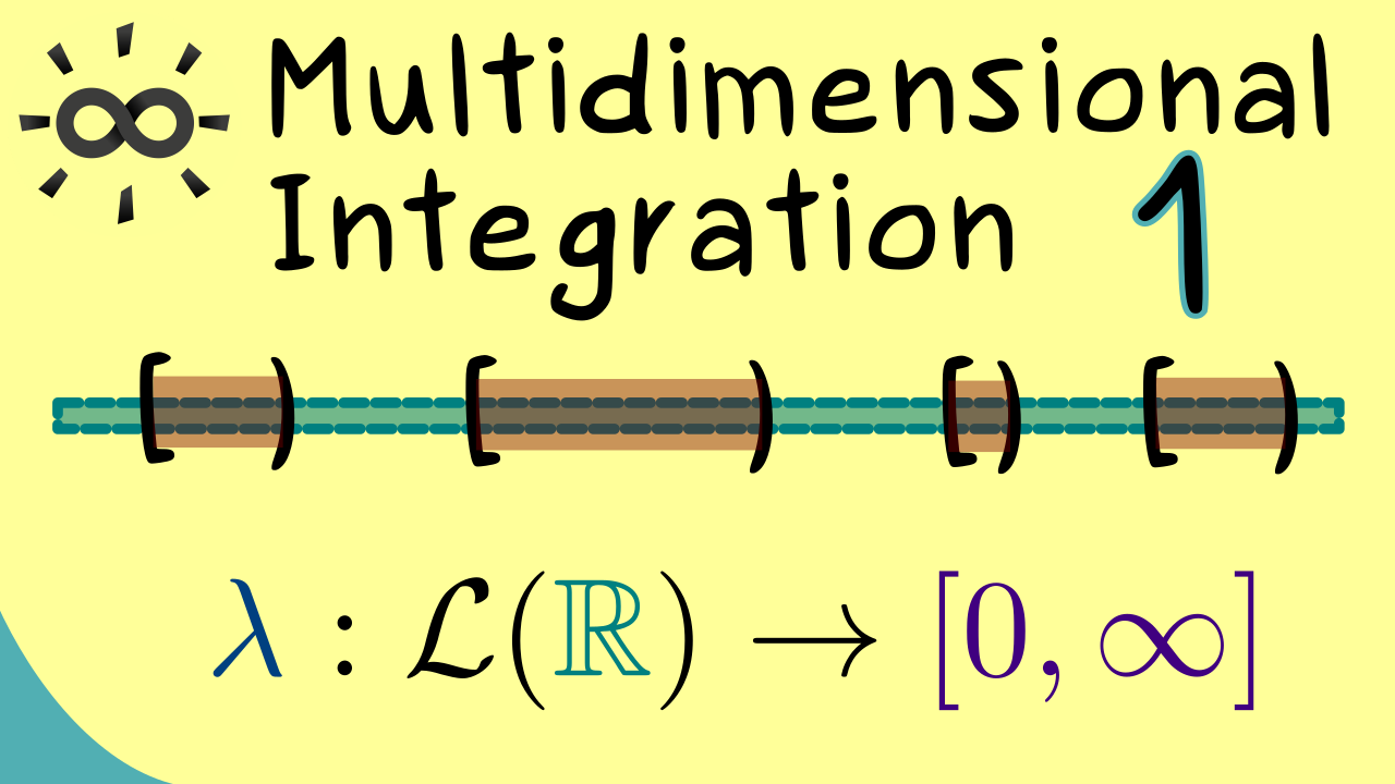
Part 1 - Lebesgue Measure and Lebesgue Integral
Let’s start the video series by stating the definition of the important Lebesgue measure. To understand the whole construction, you have to watch my Measure Theory course. However, even if you didn’t watch it, you should grasp the essential properties this measure has. The conclusion in the end is that we have a much more powerful integral on the real number line. This one generalizes the Riemann integral, you might know from Real Analysis.
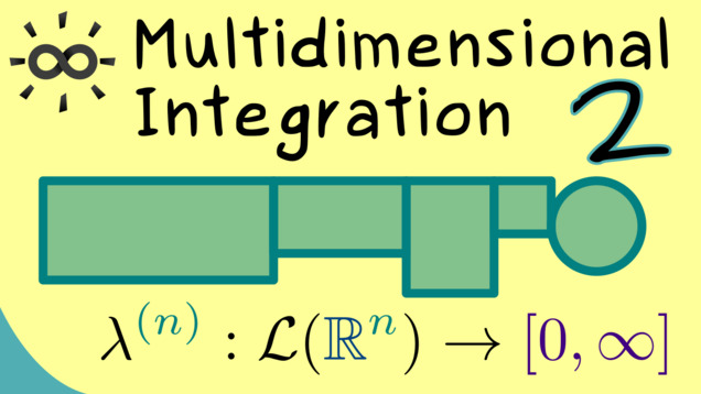
Part 2 - The n-dimensional Lebesgue Measure
In the second part, the power of the general Lebesgue integral comes really through. It’s no problem at all to generalize everything quickly to higher dimensions. This is something where the Riemann integral really struggles with, but with the Lebesgue integral, everything is simple and fast.
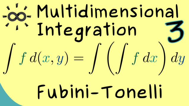
Part 3 - Fubini’s Theorem
You might already know that higher-dimensional integrals can be solved by transforming them into one-dimensional integral and solving them. This procedure is known as Fubini’s theorem or Fubini-Tonelli theorem. It works under mild assumptions for the functions such that one can say that it is really a universal tool to solve integrals. In this video, we will discuss these assumptions and the correct formulation.
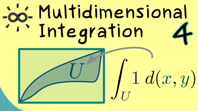
Part 4 - Fubini’s Theorem in Action
We present the usage of Fubini’s theorem by considering a simple two-dimensional example.
Part 5 - Change of Variables Formula
As an important integration technique for solving one-dimensional integrals, we know the so-called substitution rule. It turns out that one can generalize that to $n$-dimensional integrals as well and there it is known as the change of variables formula. The key ingredient there is the Jacobian determinant of a chosen diffeomorphism, often called $ \Phi $.

Part 6 - Example for Change of Variables
Let’s look at an example calculation for the change of variables formula and also for Fubini’s theorem.

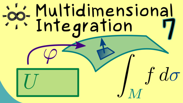
Part 7 - Surface Integral
Until now, we have only considered volume integrals in $\mathbb{R}^n$ as a generalization of the ordinary one-dimensional integral in $\mathbb{R}$. However, there is another concept of integration where you want to intgerate along a curve or over a surface. This requires a different approach for the integral because such a surface does not have be flat like $\mathbb{R}^n$. We will define this so-called surface integral by looking at tangent vectors, normal vectors, and the Gramian determinant.
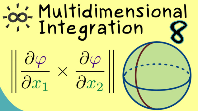
Part 8 - Example of Surface Integral
We can immediately apply the definition of the surface integral to the 2-dimensional sphere in $\mathbb{R}^3$. You might already know the spherical coordinates one can use for that. In particular, we can take them to calculate the Gramian determinant.
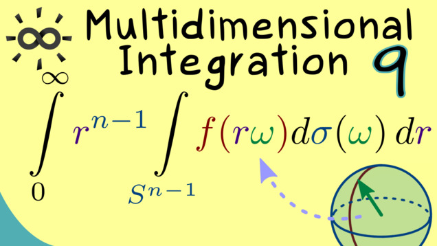
Part 9 - Integration with Polar Coordinates
While working in $\mathbb{R}^n$, it can definitely happen that a problem carries some symmetries where spherical coordinates would make the calculation easier. In the general case, this is known as integrating in polar coordinates. It turns out that the surface integral over the sphere helps a lot in formulating such an $n$-dimensional integration formula.
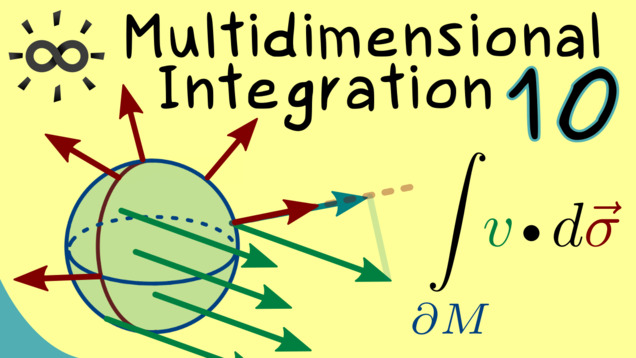
Part 10 - Divergence Theorem
A classical result in vector analysis is Gauss’s Integral Theorem also know as the Divergence Theorem because it’s connects the divergence of a vector field to a surface integral. We discuss some typical notations but don’t show the proof of this theorem since it follows from a general theorem discussed in the Manifolds series.
Other videos related to this topic:
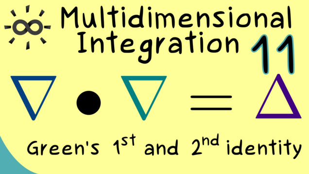
Part 11 - Green’s Identities
It turns out that the Divergence Theorem from the last video directly gives us a formula that we could call integration by parts in higher dimensions. There we see how to integrate a product of functions by shifting a derivative from one function to another one. As in the one-dimensional case, a boundary term also occurs. This is will be used to derive two statements known as Green’s first identity and Green’s seconds identity.
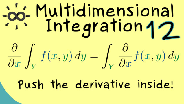
Part 12 - Differentiation Under The Integral Sign
The following video can be seen as an extension of the Measure Theory series since we just apply Lebesgue’s dominated convergence theorem. The result is that we are allowed to move the derivative inside the integral under some weak conditions. The common application of that is to use a function of several variables where the integration only happens over some variables.
Other videos related to this topic:
- Measure Theory 10 | Lebesgue’s Dominated Convergence Theorem
- Partial Differential Equations 4 | Mean-Value Property of Harmonic Functions
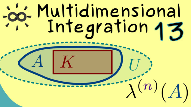
Part 13 - Lebesgue Measure is Regular
In this video series we cover a lot of different topics concerning the higher-dimensional integration. The key element there is always the Lebesgue measure on $\mathbb{R}^n$. So it’s definitely helpful to look at basic properties this measure has. One of them is the so-called regularity, which allows to approximate the value of the measure by open or compact sets of $\mathbb{R}^n$.
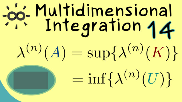
Part 14 - Proof of the Regularity of the Lebesgue Measure
After stating the regularity of the Lebesgue measure, we can try to prove it. For this we have to some work. One important part will be that every measurable set can be covered by open rectangles in $\mathbb{R}^n$.
Part 15 - Continuous Functions Are Dense in L¹
The following result is quite important: it makes a connection between integrable functions and continuous functions. Indeed, the continuous functions with compact support are definitely integrable, but now it turns out that these function are already enough to describe the whole $L^1$-space. We call this property denseness. The proof idea is not too hard: first approximate an integrable function by simple functions, and then approximate these by continuous functions. The last step can be done by Urysohn’s Lemma.
Other videos related to this topic:
- Multidimensional Integration 13 | Lebesgue Measure is Regular
- Measure Theory 10 | Lebesgue’s Dominated Convergence Theorem
- Basic Topology 11 | Urysohn’s Lemma
Part 16 - Lᵖ-Spaces
It turns out that not only the integrable functions are interesting but also the measurable functions $f$ where $|f|^p$ is integrable. The vector space of this function is denoted by $\mathcal{L}^p(\mathbb{R}^n, \mathbb{C})$. We usually choose $p \in [1, \infty)$ and define the corresponding $ \lVert \cdot \rVert_p $-norm. We can do the same procedure as for the integrable function and get a normed space of equivalence classes $(L^p(\mathbb{R}^n, \mathbb{C}), \lVert \cdot \rVert_p)$. Moreover, we can also show that the continuous functions with compact support lie dense in this space as well. The proof is more or less the same as for $L^1$.
Part 17 - Essentially Bounded Functions
Next to the $L^p$-spaces from the last videos, we can also define the $L^\infty$ space. However, there we don’t need an integral for the definition because it’s just about the essentially bounded functions. Roughly speaking, it just means that we find a bounded function in the corresponding equivalence class.
Part 18 - $L^\infty$ is Complete
One nice property of the newly defined normed vector space $L^\infty(\mathbb{R}^n, \mathbb{C} )$ is that is complete. This just means that every Cauchy sequence is actually convergent. Such a complete normed vector space is called a Banach space.
Part 19 - Riesz-Fischer Theorem
The result from the last video can actually be extended to the other $L^p$-spaces as well. This means $L^p(\mathbb{R}^n, \mathbb{C})$ is a Banach space for every $p \in [0, \infty]$.
Other videos related to this topic:
Connections to other courses
Summary of the course Multidimensional Integration
-
You can download the whole PDF here and the whole dark PDF.
-
You can download the whole printable PDF here.
- Ask your questions in the community forum about Multidimensional Integration.
Ad-free version available:
Click to watch the series on Vimeo.