Hello and welcome to my ongoing video course about Hilbert Spaces, already consisting of 24 videos. Each video is designed to guide you through the key concepts, presented in a logical order. Along with the videos, I provide clear text explanations. You can test your understanding through the quizzes and refer to the PDF versions of the lessons whenever needed. If you have any questions, the community forum is there for you. Let’s get started!
Part 1 - Introductions and Cauchy-Schwarz Inequality
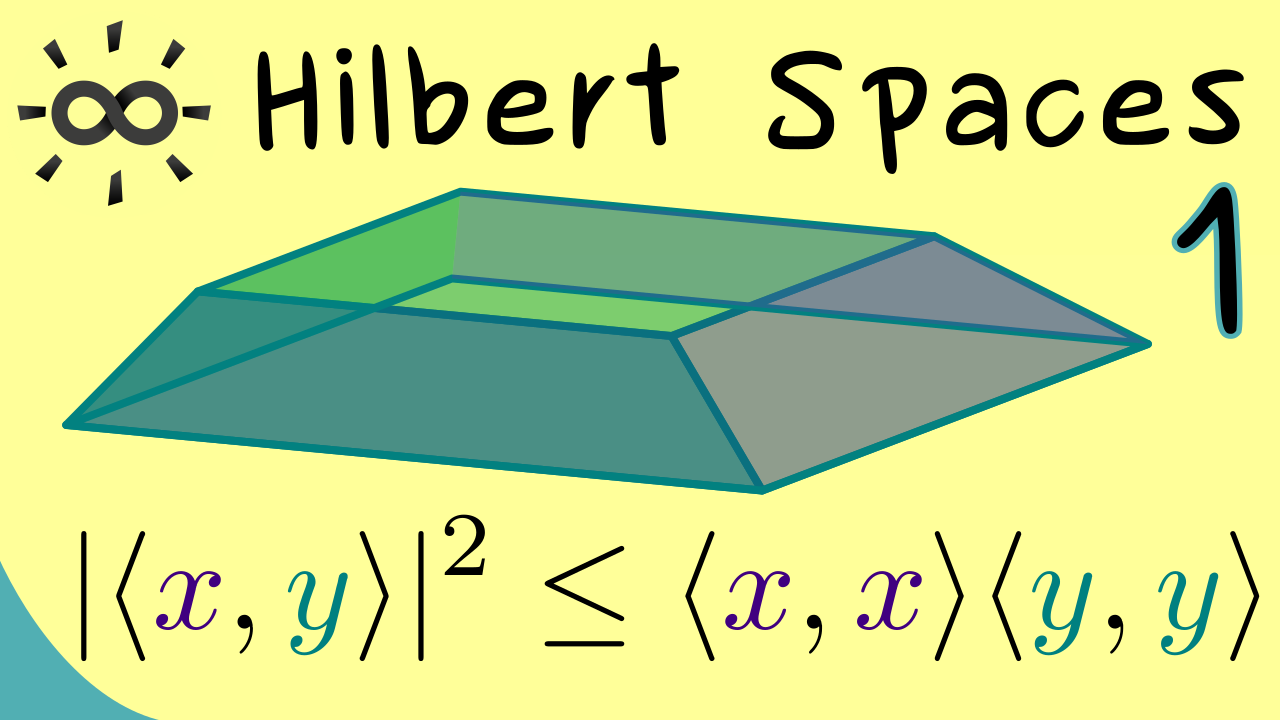
Let’s start with a short overview for the whole course and with the important definition of an inner product. This is something we have alreade discussed in Linear Algebra but now we also add an particular analysis part to it: we want to have completeness of the underlying normed space. In short, we have the following: a Hilbert space is an inner product space and a Banach space in one. We also use the first video here to prove the famous Cauchy–Bunyakovsky–Schwarz inequality.
Content of the video:
00:00 Introduction
00:45 Network for the video courses
01:40 Prerequisite for the course
02:27 Topics in Hilbert Spaces
03:53 Definition for inner product spaces
06:53 Pre-Hilbert space as an alternative name
07:11 Cauchy-Schwarz inequality
07:53 Proof of Cauchy-Schwarz
11:20 Norm on inner product spaces
11:57 Definition of Hilbert space
12:34 Credits
Part 2 - Examples of Hilbert Spaces
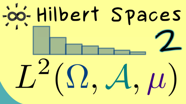
Now we are ready to look at some examples for inner product spaces which are also complete. From the Functional Analysis series, we already know the important $ \ell^2 $-space. It consists of sequences which are also square-summable. It turns out that one can generalize this example to a so-called $ L^2(\Omega, \mu) $-space. It consists of functions defined on a measure space $(\Omega, \mathcal{A}, \mu) $.
Part 3 - Polarization Identity
The polarization vividly describes what one can do with an inner product. Namely, one can decompose it into basic parts. And it turns out that the knowledge of the associated norm is enough to describe these basic parts.

Part 4 - Parallelogram Law
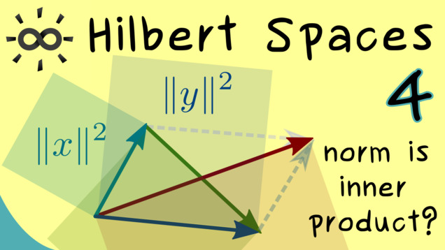
In the next video, we will discuss the parallelogram law which holds in every inner product space. However, the formulation of this formula only uses the induced norm, so the question arises if the rule can also hold in general normed spaces. It turns out that the parallelogram law actually characterizes normed spaces which are also inner product spaces.
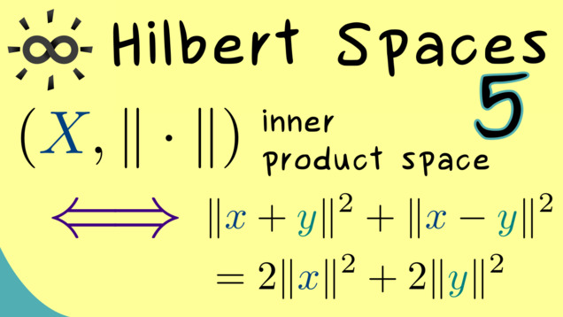
Part 5 - Proof of Jordan-von Neumann Theorem
The statement from the last video is also known as the Jordan-von-Neumann theorem. Let’s discuss the ideas of the proof of that.
Part 6 - Orthogonal Complement
The whole advantage of Hilbert spaces, and also inner product spaces in general, is that we have a geometry we can calculate with. One part of the geometry we already received: we can measure lengths with the induced norm $ | \cdot | $. However, an inner product has much more than that. We can also measure angles with it. More precisely, we can easily define what we mean by a right angle, which means that we can say when two vectors are perpendicular. This is the concept of orthogonality which every inner product space carries. Moreover, we can also define the so-called orthogonal complement for each subset in the space.

Part 7 - Approximation Formula
By using the orthogonality in inner product spaces, we can construct abstract right-angled triangles. It turns out that we also have the Pythagorean theorem in a general version there. Moreover, we should also be able to find orthogonal projections like we did in Linear Algebra. The key step for these is given by the approximation formula.

Part 8 - Proof of the Approximation Formula
Now, we are ready to prove the important approximation formula, which only holds in Hilbert spaces and not in general Banach spaces. We will see exactly that in our proof because we will use the parallelogram identity for the norm.

Part 9 - Projection Theorem
The direct application of the approximation formula leads to the existence of the orthogonal projection. Each vector can be projected to a closed subspace. This is what we call the orthogonal projection and it makes sense in every Hilbert space.

Part 10 - Orthonormal System and Orthonormal Basis
The concept of a basis for a vector space can also be used for infinite-dimensional spaces. However, it turns out that in inner product spaces, a slightly different concept is much more useful. Instead of requiring that the basis spans whole space, we only require a total set, which means that the span is only a dense subset. With this approach, we can define a total orthonormal system (ONS) that is also called orthonormal basis (ONB).

Content of the video:
00:00 Introduction
00:38 Notion: orthonormal
01:51 Definition: (infinite) ONS and ONB
03:39 Notion: total
05:00 Correction: This should hold for all ε > 0
06:20 Example: Hilbert space of sequences
09:57 Credits
Part 11 - Maximal Orthonormal Systems
An important fact in Hilbert spaces is that we can always find an orthnormal basis (ONB), also in the infinite dimensional case. We discuss the reason for this here: every maximal ONS is already an ONB. However, this nice result need the completeness of the space.

Part 12 - Bessel’s Inequality
Every ONS in a Hilbert space satisfies an important inequality that connects the Fourier coefficients $ \langle e_{\alpha} , x \rangle $ to the norm of the vector $x$. This is known as Bessel’s inequality and also used in Fourier Analysis.

Part 13 - Parseval’s Identity
It turns out that for ONBs Bessel’s inequality can be made stronger and is, in fact, an equality. We will discuss other equivalent statements which are all known as Parseval’s identity.

Part 14 - Proof of Parseval’s Identity
Let’s prove the equivalences from the last video. We do not need to assume that we have a Hilbert space, which means that the completeness is not necessary for the proof. Moreover, we also consider a general ONB of any cardinality.

Part 15 - Existence of ONB
After all these discussions about orthonormal bases, we know that they are really helpful, especially for calculating orthogonal projections. Therefore, we definitely want to guarantee that they exist for our Hilbert spaces. We can even say more, namely for every separable inner product space, we always find a countable ONB. In fact, having a separable Hilbert spaces is the common case in applications.

Part 16 - Orthogonal Projection Operators
We’ve already talked about orthogonal projections as a component of a vector in a Hilbert space with respect to a closed subspace. This procedure actually defines a linear operator $P$, which we also call orthogonal projection. They satisfy some properties. The most important one is that $P$ is idempotent.

Part 17 - Riesz Representation Theorem
From the Functional Analysis series, we already know the concept of a continuous linear functional, which is simply a bounded linear map $X \rightarrow \mathbb{F}$. This means that we map from the infinite-dimensional Hilbert space $X$ into the one-dimensional field $ \mathbb{F}$. It turns out that such a functional can always be represented by a vector $y \in X$, often denoted by $\langle y |$. This special result in Hilbert spaces is know as the Representation Theorem by Riesz. We will also prove it here.

Part 18 - Adjoint Operator
For a bounded operator $T:X \rightarrow Y$ between Hilbert spaces, there is a unique operator $T^\ast$, which we call the adjoint of $T$, and it satisfies $\langle y, T x \rangle = \langle T^\ast y, x \rangle $. In order to show this, we can use the Riesz representation theorem from the last video.

Part 19 - Properties of the Adjoint
After defining the adjoint of an operator, you might immediately see that forming the adjoint again brings us back to the original operator $T^{\ast \ast} = T$. This is exactly what you already know from Linear Algebra for matrices. However, not all properties translate so easily to infinite dimensions. In particular, if we want to write down a relation between the kernel of $T^\ast $ and the range of $T$, we need to factor in that the range is, in general, not a closed subspace.

Part 20 - Orthogonal Projections Are Self-Adjoint
After the defining the adjoint of an operator $T: X \rightarrow X$, the notion self-adjoint is quite self-explanatory. It simply means $T^\ast = T$. Going back to orthogonal projection operators, we can show that these are always self-adjoint. Moreover, idempotent and self-adjoint are exactly the defining properties of an orthogonal projection.

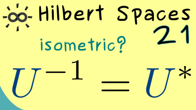
Part 21 - Unitary Operators
There are also other important operators that are usually not self-adjoint. One special kind is given by so-called unitaries. These are actually the isomorphisms of Hilbert spaces, which means they need to be bijective and conserve lengths and angles. Since we have the polarization identity, it’s enough to claim that the norm does not change under map. This is what we call an isometry. Let’s put this into the definition of a unitary operator:
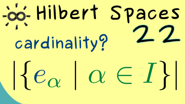
Part 22 - Hilbert Space Dimension
In Linear Algebra, the dimension of a vector space is defined as the cardinality of a basis. We can do a similar thing for Hilbert spaces. The Hilbert space dimension is just the cardinality of an orthonormal basis. Please note that these two notions only overlap in finite dimensions. However, now it turns out that the Hilbert Space dimension already determines the Hilbert space completely, which means that Hilbert spaces with the same space Hilbert space dimension are isomorphic.
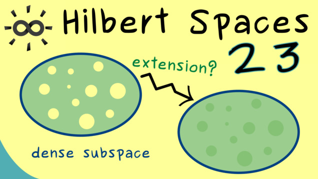
Part 23 - Extension of Isometries
A linear map that conserves the norm is called an isometry. So a unitary operator is always an isometry but the converse is not true in general. In this video, we will extend an isometry defined on a dense subspace to an isometry defined on the whole Hilbert space. This always works in a unique way.
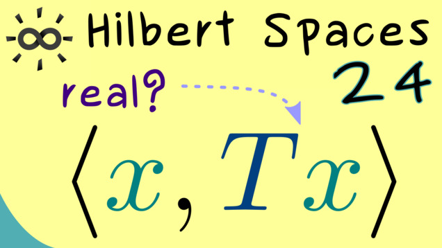
Part 24 - Self-Adjoint Operators
Connections to other courses
Summary of the course Hilbert Spaces
-
You can download the whole PDF here and the whole dark PDF.
-
You can download the whole printable PDF here.
- Ask your questions in the community forum about Hilbert Spaces.
Ad-free version available:
Click to watch the series on Vimeo.