1 00:00:00,500 –> 00:00:05,808 Hello and welcome back to the video series about ODEs.

2 00:00:06,386 –> 00:00:14,542 So you see we are still in the beginning of the topic and in today’s part 2 we will first define the important notions we need.

3 00:00:14,742 –> 00:00:20,307 So for example we will give the definition what we mean by an ODE.

4 00:00:20,507 –> 00:00:27,583 However, before we do that I first want to thank all the nice people who support this channel on Steady, via Paypal or by other means

5 00:00:28,243 –> 00:00:34,778 and please don’t forget, in the description you find the link, where you can download the PDF version and a quiz for this video.

6 00:00:34,978 –> 00:00:41,121 Ok, then without further ado let’s start with the important definitions we will need in this series.

7 00:00:41,586 –> 00:00:46,674 First of all we will often deal with a set of functions called C^k

8 00:00:46,874 –> 00:00:52,418 and usually the domain of definition for these functions is given by an interval “I”.

9 00:00:52,771 –> 00:00:57,890 Hence when you see capital “I” it’s always a subset of the real number line.

10 00:00:58,529 –> 00:01:06,376 Now in fact most of the time in this series it will denote an interval, but sometimes it will denote a general open set

11 00:01:06,771 –> 00:01:12,196 and in some other cases we might want that “I” stands for a union of 2 intervals.

12 00:01:12,396 –> 00:01:17,736 So you see, depending on what we want to do later, we will stretch this definition a little bit,

13 00:01:17,737 –> 00:01:20,557 but here we will start with an interval “I”

14 00:01:20,884 –> 00:01:25,901 and then this set C^k is well-defined as a set of functions

15 00:01:26,371 –> 00:01:34,398 and here we immediately see the first special feature of this topic, because we will denote functions by a lower case x.

16 00:01:34,900 –> 00:01:39,556 Hence x is a function, where the domain of definition is “I”

17 00:01:39,986 –> 00:01:43,168 and it simply maps into the real number line

18 00:01:43,900 –> 00:01:52,380 and now you should recall from real analysis that C^k means that the function x is k-times continuously differentiable.

19 00:01:52,914 –> 00:01:58,895 This means the kth order derivative of x exists and is a continuous function.

20 00:01:59,095 –> 00:02:06,205 Moreover I should tell you here that the variable name we want to use for the function x is usually a lower case t.

21 00:02:06,614 –> 00:02:09,623 This means we will write x(t).

22 00:02:09,823 –> 00:02:16,809 I tell you that, because if we choose the variable name as t, we will use a dot for denoting derivatives.

23 00:02:17,271 –> 00:02:21,583 Hence the first derivative here would be the function x dot.

24 00:02:21,783 –> 00:02:25,390 Then the second derivative would be x dot dot

25 00:02:25,590 –> 00:02:31,659 and so on and of course if we need too many dots, we will use the common upper index notation.

26 00:02:32,186 –> 00:02:37,904 Of course in situations where the dot could be confusing, we will just use other notations.

27 00:02:38,104 –> 00:02:42,785 So for example you know the common prime notation or the Leibniz notation.

28 00:02:42,985 –> 00:02:47,789 So please keep that in mind. Depending on the context or depending on which book you read,

29 00:02:47,989 –> 00:02:51,072 you will see different notations for the derivative.

30 00:02:51,529 –> 00:02:56,621 However the definition for an ODE should be the same.

31 00:02:57,171 –> 00:03:02,496 Namely it should be given by a combination of the derivatives of the function x.

32 00:03:02,971 –> 00:03:06,466 Indeed, we could write it down by a functional relation.

33 00:03:06,666 –> 00:03:10,116 For that we take a continuous function capital F

34 00:03:11,014 –> 00:03:15,694 and then we have different inputs. First of all the independent variable t

35 00:03:15,894 –> 00:03:20,941 and then the function x and the derivatives of x up to some order.

36 00:03:21,141 –> 00:03:25,886 So as before we could say that the highest derivative is the kth order.

37 00:03:26,271 –> 00:03:30,447 Ok and now this function with all the inputs should be equal to 0.

38 00:03:30,971 –> 00:03:38,368 Ok, so you see in general this is what we mean when we talk of an ODE of order k

39 00:03:38,643 –> 00:03:42,938 and maybe let’s immediately look at an example for such an equation.

40 00:03:43,357 –> 00:03:52,864 So we could have t + x + 2xdot + second derivative of x squared

41 00:03:53,686 –> 00:03:56,339 and then this should be equal to 0.

42 00:03:56,800 –> 00:04:02,563 So there you see, this is a well defined ODE of second order.

43 00:04:02,763 –> 00:04:07,900 So the highest derivative that occurs in the equation gives us the order

44 00:04:08,114 –> 00:04:15,831 and at this point you might say, it might be easier for us if we first start with first order differential equations.

45 00:04:16,329 –> 00:04:22,728 In fact soon we will see why it’s very helpful to start with the first order differential equations.

46 00:04:23,271 –> 00:04:29,666 Ok, but now it’s helpful for the next definitions to abbreviate the term ordinary differential equation.

47 00:04:30,286 –> 00:04:36,312 From now on we will simply write ODE if we need to keep it short and compact.

48 00:04:36,771 –> 00:04:42,129 Therefore in the next definition we will explain explicit ODEs of order 1.

49 00:04:42,871 –> 00:04:49,051 Here explicit means that the derivative we are interested in is on the one side of the equation

50 00:04:49,251 –> 00:04:54,417 and all the other terms like the function x and the variable t are on the other side

51 00:04:54,914 –> 00:04:59,054 and both things we can rewrite with a function w.

52 00:04:59,254 –> 00:05:02,895 Hence w gets 2 inputs, t and x.

53 00:05:03,095 –> 00:05:08,202 Moreover we would say w is a function defined on 2 intervals.

54 00:05:08,800 –> 00:05:13,075 So we have the interval “I” for t and the interval J for x

55 00:05:13,771 –> 00:05:18,376 and in this case here both are simply intervals from the real number line.

56 00:05:18,900 –> 00:05:25,192 Ok, so in summary you see here, this one is a special case of our general case from above.

57 00:05:25,392 –> 00:05:28,569 However it’s the common one we will examine.

58 00:05:29,000 –> 00:05:34,235 That’s because the 2 restrictions we have here are actually not big restrictions.

59 00:05:34,857 –> 00:05:39,304 Indeed we will discuss soon why this case here is very general,

60 00:05:39,504 –> 00:05:44,967 but first I would say let’s look at an example of an explicit ODE of order 1.

61 00:05:45,167 –> 00:05:49,516 Hence we already know, on the left-hand side we need to have x dot

62 00:05:49,716 –> 00:05:54,374 and now on the right-hand side for example we could have x + t

63 00:05:54,629 –> 00:05:58,868 So you see, the function w doesn’t have to be very complicated.

64 00:05:59,643 –> 00:06:04,066 In fact here the domain of definition is simply R^2.

65 00:06:04,557 –> 00:06:10,085 Ok, but at this point you might remember what we have discussed in the last video.

66 00:06:10,285 –> 00:06:15,048 There we had examples where more than 1 variable were involved.

67 00:06:15,600 –> 00:06:21,533 Therefore we might ask: “is there also an example here for an explicit ODE of order 1?”

68 00:06:21,733 –> 00:06:30,570 So you could write x_1 dot, the first variable for x is equal to the second variable x_2 + t

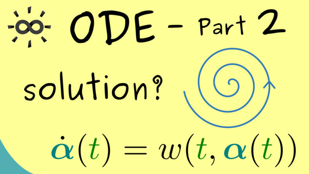
69 00:06:30,770 –> 00:06:34,830 and then we could have a similar equation for x_2 dot.

70 00:06:35,030 –> 00:06:38,362 Now this one could be x_1 + t.

71 00:06:38,562 –> 00:06:45,405 Now, important to note here is, these are not just 2 individual ODEs of order 1.

72 00:06:45,786 –> 00:06:49,950 Otherwise it would not be allowed to mix the variables in this way.

73 00:06:50,286 –> 00:06:54,988 However we can just put them together and call it a system of ODEs

74 00:06:55,188 –> 00:06:59,644 and in fact a system of ODEs looks exactly the same again.

75 00:07:00,143 –> 00:07:03,205 We simply have to write it as a vector equation.

76 00:07:03,686 –> 00:07:11,365 So the derivative of the vector x_1, x_2 is equal to a vector given by the right-hand side here

77 00:07:11,565 –> 00:07:16,561 and of course this one can be expressed again by a function w.

78 00:07:16,761 –> 00:07:23,558 So w gets again 2 inputs, but now the second input is a vector instead of the variable x

79 00:07:23,758 –> 00:07:31,301 and then you should see, if we call the vector (x_1, x_2) simply x again, it has the same form as before.

80 00:07:31,871 –> 00:07:37,124 In other words now we are able to define the term system of ODEs.

81 00:07:37,324 –> 00:07:45,601 More precisely you would say we have an n-dimensional system of explicit ODEs of order 1,

82 00:07:45,929 –> 00:07:52,086 but you might already know in the end we will also just say ODE for such a system.

83 00:07:52,286 –> 00:07:57,760 Simply because from the form, from the looks it’s the same as our original definition.

84 00:07:58,129 –> 00:08:02,835 However don’t forget, the value x(t) is now a vector.

85 00:08:03,035 –> 00:08:06,881 More precisely we would say it’s a n-dimensional vector.

86 00:08:07,371 –> 00:08:11,929 So in other words our system now could have n equations here.

87 00:08:12,529 –> 00:08:16,544 Hence the function w now also maps into R^n.

88 00:08:17,229 –> 00:08:21,797 Moreover the domain of definition also changes for the second variable.

89 00:08:22,471 –> 00:08:27,094 Usually we would say we have U there, which is an open set in R^n,

90 00:08:27,429 –> 00:08:34,277 but as we said at the beginning also that changes a little bit depending which problem we consider.

91 00:08:35,114 –> 00:08:41,280 Ok, but for the moment I would say we have a very nice definition for what we mean when we say ODE.

92 00:08:41,480 –> 00:08:47,661 So this is a very general construct, but you see one important ingredient is still missing here.

93 00:08:48,243 –> 00:08:56,693 So now we know what an ODE is, but we remember for applications we are always interested in solutions of this ODE.

94 00:08:56,893 –> 00:09:02,893 So know the question is: what is a solution of a system of ODEs?

95 00:09:03,414 –> 00:09:09,268 Of course it should be a function that is differentiable and can be put into the equation

96 00:09:09,468 –> 00:09:13,656 and then it should fulfill the equation for all points t.

97 00:09:13,856 –> 00:09:20,073 However there you already see, the domain of definition doesn’t have to be the whole interval “I”.

98 00:09:20,386 –> 00:09:25,901 Indeed, it could be any subinterval which we can call t_0 to t_1.

99 00:09:26,101 –> 00:09:31,930 So this is an open interval and now the solution function we can simply call alpha.

100 00:09:32,543 –> 00:09:37,268 So alpha is defined on this interval and it maps into R^n.

101 00:09:37,468 –> 00:09:41,360 More precisely it has to map into the subset U.

102 00:09:42,029 –> 00:09:49,242 Simply because we want to put it into our function w in the second component and then it should be well-defined.

103 00:09:49,886 –> 00:09:54,407 Ok, there we have it. Solution means it fulfills this equation here.

104 00:09:54,714 –> 00:10:06,152 More concretely the derivative of alpha at the point t is equal to w(t, alpha(t)).

105 00:10:06,600 –> 00:10:14,155 So there you see this is a well-defined equation of vectors and it should be fulfilled for all t in the interval.

106 00:10:14,414 –> 00:10:18,969 So you see, now we can check this condition here pointwisely

107 00:10:19,343 –> 00:10:24,716 and most importantly you should see the solution is always a differentiable function.

108 00:10:25,371 –> 00:10:32,336 Ok, so we have a lot of definitions here. Therefore let’s close the video now with a concrete example.

109 00:10:32,843 –> 00:10:38,882 So this one should be very helpful to see what it really means to be a solution for an ODE

110 00:10:39,082 –> 00:10:43,314 and for this let’s look at a very simple system of ODEs.

111 00:10:43,771 –> 00:10:49,487 x_1 dot should be equal to x_2 and x_2 dot should be equal to -x_1.

112 00:10:50,171 –> 00:10:54,787 So you see this is a well-defined system for n=2

113 00:10:54,987 –> 00:11:00,463 and moreover we don’t have a problem with the domain of definition. U is simply R^2

114 00:11:00,663 –> 00:11:06,822 and then the function w(t, x) is equal to x_2, -x_1.

115 00:11:07,022 –> 00:11:11,951 So you see w does not explicitly depend on t,

116 00:11:12,151 –> 00:11:17,927 but please don’t forget t comes in again if you put in the solution alpha(t).

117 00:11:18,571 –> 00:11:23,614 Ok, so now if you look at a system, maybe you immediately see a solution.

118 00:11:23,814 –> 00:11:29,256 Indeed, I know sine and cosine functions fulfill something like that.

119 00:11:29,456 –> 00:11:35,923 In fact alpha(t) = (sin(t), cos(t)) does the job.

120 00:11:36,243 –> 00:11:44,287 Simply because we know the derivative of sine is the cosine and the derivative of the cosine is the -sine function.

121 00:11:45,143 –> 00:11:49,578 Hence we immediately have a solution of this system of ODEs

122 00:11:50,300 –> 00:11:55,173 and know what one can do is to sketch the solution as its image.

123 00:11:55,629 –> 00:12:00,969 So we know the image of the solution lives in U, which is R^2 in this case

124 00:12:01,386 –> 00:12:08,893 and now we can sketch what happens to alpha(t) when we start at t=0 and then increase t.

125 00:12:09,243 –> 00:12:13,923 In fact you see what we get is a nice circle with radius 1.

126 00:12:14,357 –> 00:12:14,388 .

127 00:12:14,743 –> 00:12:20,970 Moreover now you can remember this image of the solution is called the orbit of the solution.

128 00:12:21,170 –> 00:12:28,331 Indeed it’s a dynamic picture that tells us what happens to the solution in the time variable t.

129 00:12:28,657 –> 00:12:33,592 Moreover now you should also see that we easily find a second solution here.

130 00:12:34,186 –> 00:12:42,728 Namely if we scale the vector by 1/2 and call the solution alpha tilde, then we see the ODE is also fulfilled

131 00:12:42,928 –> 00:12:47,826 and there we get that the orbit is a circle with radius 1/2.

132 00:12:48,486 –> 00:12:55,110 Hence our first result here is that a system of ODEs can have a lot of different solutions.

133 00:12:55,786 –> 00:13:00,976 Therefore a question should also be: which solution gives us the correct picture?

134 00:13:01,176 –> 00:13:07,096 Or more precisely maybe we want the solution that goes through some particular points

135 00:13:07,771 –> 00:13:14,966 and there we immediately have the questions: Do we have a solution that goes through the points and if we have it, is it unique?

136 00:13:15,657 –> 00:13:19,813 and exactly these questions we want to answer in this video course.

137 00:13:20,314 –> 00:13:27,103 Therefore I hope that you are not scared off by all these definitions and come back to the next video.

138 00:13:27,303 –> 00:13:33,742 There we will make more geometric pictures, such that you can understand the theory visually.

139 00:13:36,186 –> 00:13:37,800 So I hope we meet again and have a nice day. Bye!

Q1: Is the equation given by $$ \sin(\dot{x}) + (\ddot{x})^4 + \dddot{x} + t^5 = 0$$ an ordinary differential equation?

A1: Yes!

A2: No!

A3: One needs more information.

Q2: Is the equation given by $$ \frac{1}{(\ddot{x})^4} + t^5 = 0$$ an ordinary differential equation?

A1: Yes!

A2: No!

A3: One needs more information.

Q3: Is the equation given by $$ \sin(\dot{x}) = t^3 $$ an explicit ordinary differential equation of first order?

A1: Yes!

A2: No!

A3: One needs more information.

Q4: What is not a solution of the ODE $$ \dot{x} = \sin(x) $$

A1: $\alpha(t) = 0$ for all $ t \in \mathbb{R}$?

A2: $\alpha(t) = \pi$ for all $ t \in \mathbb{R}$?

A3: $\alpha(t) = \cos(t)$ for all $ t \in \mathbb{R}$?

A4: $\alpha(t) = -\pi$ for all $ t \in \mathbb{R}$?