
-
Title: Reducing to First Order
-
Series: Ordinary Differential Equations
-
Chapter: The Language of ODEs
-
YouTube-Title: Ordinary Differential Equations 4 | Reducing to First Order
-
Bright video: Watch on YouTube
-
Dark video: Watch on YouTube
-
Ad-free video: Watch Vimeo video
-
Forum: Ask a question in Mattermost
-
Quiz: Test your knowledge
-
Dark-PDF: Download PDF version of the dark video
-
Print-PDF: Download printable PDF version
-
Thumbnail (bright): Download PNG
-
Thumbnail (dark): Download PNG
-
Subtitle on GitHub: ode04_sub_eng.srt
-
Download bright video: Link on Vimeo
-
Download dark video: Link on Vimeo
-
Timestamps (n/a)
-
Subtitle in English
1 00:00:00,443 –> 00:00:05,557 Hello and welcome back to the video series about ODEs.
2 00:00:06,200 –> 00:00:10,882 It’s a long name and therefore often we just say ODE
3 00:00:11,343 –> 00:00:19,114 and in today’s part 4 we will show that any system of ODEs can be reduced to a first order system.
4 00:00:19,571 –> 00:00:27,369 This is very helpful, because it means that we can describe the theory just with first order ODEs.
5 00:00:27,757 –> 00:00:34,418 It also means that we can always use this nice directional field we have introduced in the last video.
6 00:00:34,871 –> 00:00:38,200 Ok, but before we start with the formulas, you already know,
7 00:00:38,329 –> 00:00:43,707 first I want to thank all the nice people, who support this channel on Steady, via Paypal or by other means.
8 00:00:44,243 –> 00:00:49,010 Only because of your support I’m able to create such video courses here
9 00:00:49,300 –> 00:00:55,886 and please don’t forget you can download the PDF version and the quiz for this video, with the link in the description.
10 00:00:56,229 –> 00:01:00,386 Ok, then let’s start with the topic of today by looking at an example.
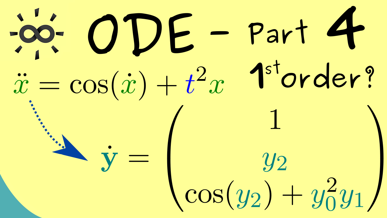
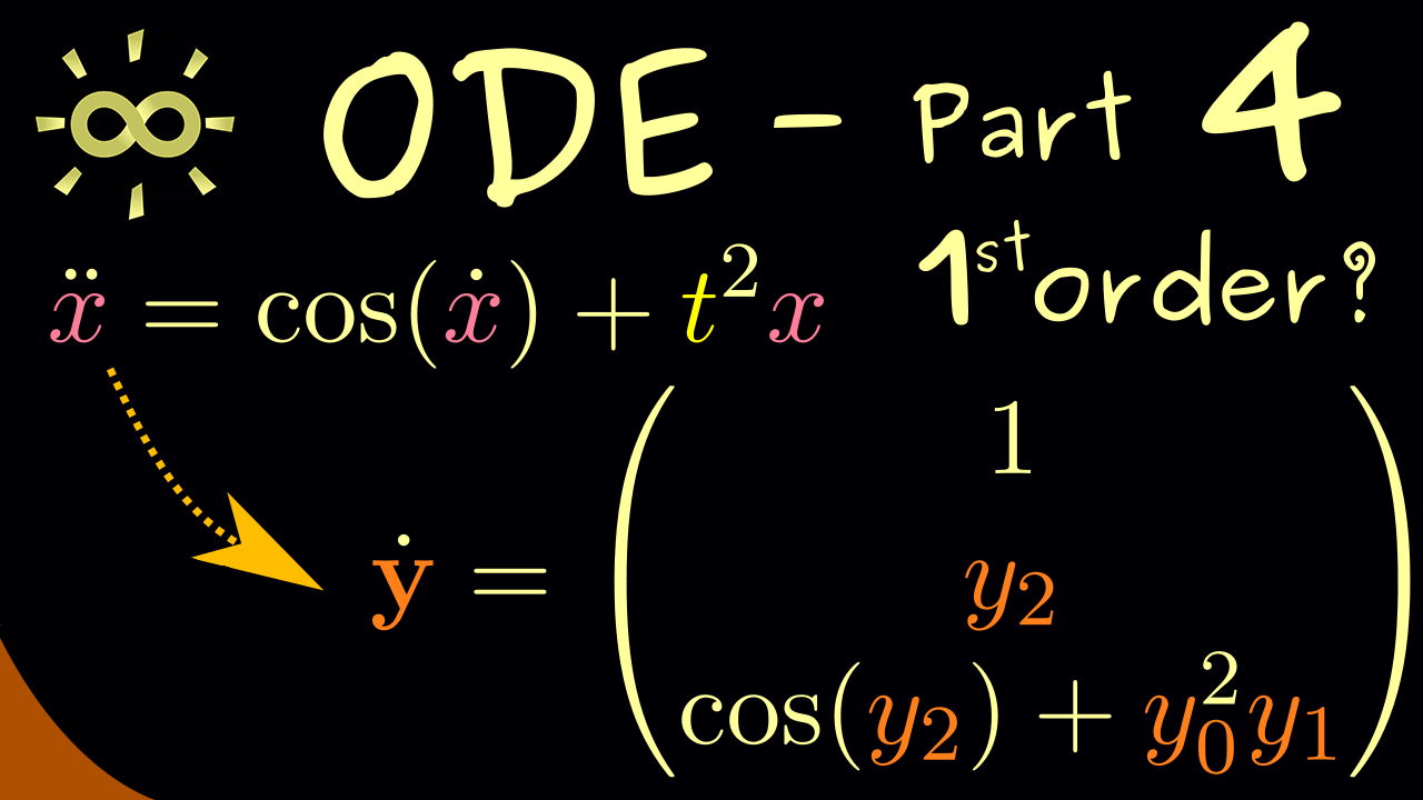
11 00:01:00,914 –> 00:01:05,216 We choose that the highest derivative we have is the third derivative
12 00:01:05,943 –> 00:01:10,366 and then this should be equal to the cosine of the second derivative.
13 00:01:11,100 –> 00:01:14,879 Plus first derivative squared + x.
14 00:01:15,271 –> 00:01:20,249 So this is what we would call an explicit ODE of third order.
15 00:01:20,686 –> 00:01:27,890 Moreover the time variable t is not involved on the right-hand side here. So it’s a so called autonomous ODE.
16 00:01:28,229 –> 00:01:34,643 and now I will show that we can reduce this ODE to a system of ODEs of first order
17 00:01:34,843 –> 00:01:42,090 and this simply works by defining a vector variable y that has the derivatives of x as components.
18 00:01:42,843 –> 00:01:51,743 More precisely the first component should be x, then comes x dot and the last component, the third component is x dot dot.
19 00:01:52,571 –> 00:01:59,320 So you see, all the functions x here on the right-hand side are now written as components of a vector.
20 00:01:59,743 –> 00:02:04,421 So instead of 3 functions, we now have 1 vector with 3 components
21 00:02:04,621 –> 00:02:12,658 and now the idea is that we can rewrite the original ODE, the equation from above, with the help of the components of y.
22 00:02:12,858 –> 00:02:19,630 So this means that the third derivative of x is now the first derivative of the third component of y
23 00:02:20,071 –> 00:02:25,301 and then on the right-hand side we can also substitute all variables x.
24 00:02:25,501 –> 00:02:34,240 Again, the second derivative here is our y_3 and the first derivative is y_2 and x itself is y_1.
25 00:02:34,943 –> 00:02:41,145 There you see, this is the whole idea. Now the first derivative is the highest order that occurs.
26 00:02:41,714 –> 00:02:46,477 However now we also have to make the connections between the other components.
27 00:02:46,829 –> 00:02:51,122 So you see y_2 dot is equal to y_3
28 00:02:51,322 –> 00:02:55,663 and lastly we have that y_1 dot is equal to y_2.
29 00:02:56,000 –> 00:02:58,575 Ok and there you see, this is all.
30 00:02:58,657 –> 00:03:07,417 This system of 3 equations has exactly the same information as this one ODE, where we have a third order for the derivative.
31 00:03:08,143 –> 00:03:18,131 However this was the whole idea, because now we can simply write y dot is equal to a vector function v(y).
32 00:03:18,729 –> 00:03:23,599 So know you see we have a nice system of ODEs of first order.
33 00:03:23,986 –> 00:03:33,694 So we conclude if we understand in general the system of first order ODEs, we can also understand higher order ODEs.
34 00:03:34,257 –> 00:03:42,070 However at this point you should ask: what can we do, if we have a system or an ODE which is not autonomous?
35 00:03:42,614 –> 00:03:46,255 For this let’s simply look at the next example.
36 00:03:46,455 –> 00:03:52,743 So let’s say we have a similar example as before, but now also t occurs on the right-hand side.
37 00:03:52,943 –> 00:03:56,064 So maybe we find -t to the power 4 here.
38 00:03:56,729 –> 00:04:01,828 Hence this is now a non-autonomous ODE, but still of third order.
39 00:04:02,314 –> 00:04:09,551 Therefore we could do the same procedure as before to get it to first order, but still it would be non-autonomous.
40 00:04:10,200 –> 00:04:14,650 So we have to do one step more to get rid of this t here.
41 00:04:15,057 –> 00:04:20,408 Indeed, we could do exactly the same as before and define the vector y as above.
42 00:04:20,943 –> 00:04:25,690 However now we also have to put in the variable t in some sense
43 00:04:26,329 –> 00:04:31,942 and one thing that works very nicely is to use it as the first variable here in the vector
44 00:04:32,486 –> 00:04:37,824 and if you want to keep the Indices as before, we should call it the 0th component.
45 00:04:38,100 –> 00:04:44,187 In other words our vector y has 4 components, where we start counting with 0.
46 00:04:44,614 –> 00:04:48,543 So we start with y_0, then we have y_1, y_2 and so on.
47 00:04:49,229 –> 00:04:53,087 Indeed if we do that, we can do exactly the same as above.
48 00:04:53,700 –> 00:04:58,456 In other words these 3 equations from above, we can just copy here.
49 00:04:58,857 –> 00:05:03,713 The only thing to add is now, in the last equation, our 0th component.
50 00:05:04,200 –> 00:05:07,965 So t to the power 4 is now y_0 to the power 4.
51 00:05:08,571 –> 00:05:14,167 In other words this is now autonomous, because there is no t on the right-hand side anymore.
52 00:05:14,571 –> 00:05:20,179 However this means we have to introduce a new equation to describe our t,
53 00:05:20,586 –> 00:05:26,515 but of course this is very simple, because we can simply calculate the derivative of t.
54 00:05:26,715 –> 00:05:30,657 So we see y_0 dot is equal to 1.
55 00:05:30,986 –> 00:05:37,617 So in the end we see, this does not change anything. It does not make the ODEs simpler our easier to solve,
56 00:05:37,817 –> 00:05:44,951 but we see we can transform a non-autonomous ODE into a system of autonomous ODEs.
57 00:05:45,343 –> 00:05:52,661 Hence in short, all explicit ODEs can be described with this formula here.
58 00:05:53,157 –> 00:05:57,677 The only thing that might change is the number of components of y.
59 00:05:57,877 –> 00:06:05,952 So this is definitely we should remember, because it explains why in our theory here we only consider this form.
60 00:06:06,600 –> 00:06:09,940 So I would say let’s write this down in general terms.
61 00:06:10,271 –> 00:06:14,257 Now assume we have an autonomous ODE of nth order.
62 00:06:14,714 –> 00:06:19,584 Then we can do the substitution as before and get a system of first order.
63 00:06:19,784 –> 00:06:23,785 However now the variable y has n components.
64 00:06:24,257 –> 00:06:30,033 So in summary we get an autonomous system of n ODEs of first order
65 00:06:30,233 –> 00:06:35,310 and now you know, we can do exactly the same, if we have a non-autonomous ODE.
66 00:06:35,986 –> 00:06:45,151 We simply do the substitution as explained here. Which means we get a system of ODEs, but y now has n+1 components.
67 00:06:45,657 –> 00:06:52,399 Ok, there we have it. The result here is again an autonomous system of ODEs of first order
68 00:06:52,971 –> 00:07:00,018 and this explains why in theorems and propositions we will always take this form for a general ODE.
69 00:07:00,218 –> 00:07:06,300 It’s not a restriction at all, because we can always translate back to the original ODE.
70 00:07:06,686 –> 00:07:14,713 So for example if we have found a solution here on the right-hand side we can simply translate it to a solution for the left-hand side.
71 00:07:15,071 –> 00:07:20,014 This is no problem at all, because you see the translation here is very simple.
72 00:07:20,286 –> 00:07:29,285 Ok, I would say in order to get some practice for dealing with ODEs, we will look at some methods for solving them in the next video.
73 00:07:29,843 –> 00:07:35,453 Of course finding solutions is a very important part of this theory here.
74 00:07:35,771 –> 00:07:40,222 Therefore I hope I see you in the next video and have a nice day. Bye!
-
Quiz Content
Q1: Consider the ODE given by $$ \dot{x} + t^5 = 5$$ What is the corresponding autonomous system of ODEs of first order?
A1: $$ \begin{matrix} \dot{y}_0 = 1 \ \dot{y}_1 = 5 - y_0^5 \end{matrix} $$
A2: $$ \begin{matrix} \dot{y} = 5 - y^5 \end{matrix} $$
A3: $$ \begin{matrix} \dot{y}_0 = 1 \ \dot{y}_1 = 5 \end{matrix} $$
A4: $$ \begin{matrix} \dot{y}_0 = 0 \ \dot{y}_1 = 5 + y_0^5 \end{matrix} $$
Q2: Consider the ODE given by $$ \ddot{x} = \dot{x} - 1 +x$$ What is the corresponding autonomous system of ODEs of first order?
A1: $$ \begin{matrix} \dot{y}_1 = y_2 \ \dot{y}_2 = y_2 -1 + y_1 \end{matrix} $$
A2: $$ \begin{matrix} \dot{y} = 5 - y^5 \end{matrix} $$
A3: $$ \begin{matrix} \dot{y}_1 = - y_2 \ \dot{y}_2 = y_1 -1 + y_2 \end{matrix} $$
A4: $$ \begin{matrix} \dot{y}_1 = y_2 \ \dot{y}_2 = y_1 -1 + y_2 \end{matrix} $$
-
Last update: 2025-08