
-
Title: Introduction (including R)
-
Series: Probability Theory
-
YouTube-Title: Probability Theory 1 | Introduction (including R)
-
Bright video: Watch on YouTube
-
Dark video: Watch on YouTube
-
Ad-free video: Watch Vimeo video
-
Forum: Ask a question in Mattermost
-
Quiz: Test your knowledge
-
Dark-PDF: Download PDF version of the dark video
-
Print-PDF: Download printable PDF version
-
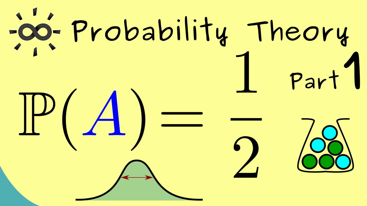
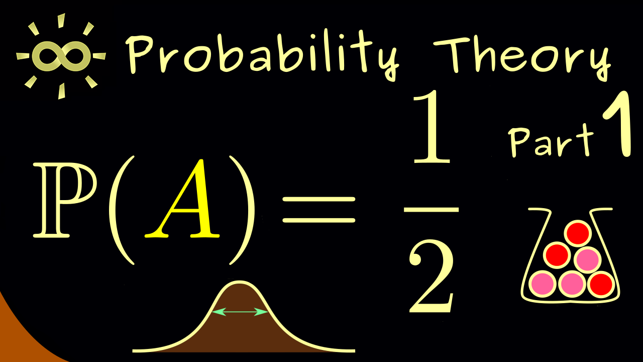
R file: Download R file
-
Exercise Download PDF sheets
-
Thumbnail (bright): Download PNG
-
Thumbnail (dark): Download PNG
-
Subtitle on GitHub: pt01_sub_eng.srt
-
Download bright video: Link on Vimeo
-
Download dark video: Link on Vimeo
-
Timestamps
00:00 Introduction
01:20 simple example: throwing a die
02:54 Rstudio
05:17 Outro
-
Subtitle in English
1 00:00:00,150 –> 00:00:03,340 Hello and welcome to probability theory.
2 00:00:03,550 –> 00:00:07,240 A video series where we want to talk about stochastic problems.
3 00:00:08,000 –> 00:00:13,500 The making of this new course is only possible, because of very nice supporters on Steady and Paypal.
4 00:00:14,220 –> 00:00:17,610 Therefore thank you very much and i hope you enjoy the videos.
5 00:00:18,110 –> 00:00:22,600 And for the start i can tell you the goal of probability theory in general
6 00:00:22,680 –> 00:00:27,970 is to formalize things like randomness and chances to get a mathematical theory.
7 00:00:28,440 –> 00:00:33,130 So you see the topics here could be very applied, but it’s still mathematics.
8 00:00:33,890 –> 00:00:38,710 Also i can tell you there are a lot of different names this course could have alternatively.
9 00:00:38,920 –> 00:00:44,270 For example we could call it Stochastic, stochastic processes or even statistics.
10 00:00:44,870 –> 00:00:51,350 However, because i want to cover a lot of different topics here i stay with the very general probability theory.
11 00:00:51,830 –> 00:00:57,350 To get an idea what to expect here i have some notions and topics in these boxes for you.
12 00:00:57,860 –> 00:01:03,640 For example we will describe what a Probability measure or a Probability distribution really is.
13 00:01:03,900 –> 00:01:05,700 So measure theory comes in.
14 00:01:06,470 –> 00:01:12,460 Then random variables and random processes are needed to describe a lot of random experiments.
15 00:01:12,850 –> 00:01:16,840 Also i think it’s very important to prove the central limit theorem
16 00:01:16,860 –> 00:01:19,640 and apply all our knowledge to statistical tests.
17 00:01:20,520 –> 00:01:25,610 Ok i would say before diving into the whole theory let’s look at a simple example.
18 00:01:26,630 –> 00:01:31,220 So maybe not so surprising. Just let’s throw a normal 6 sided die.
19 00:01:31,920 –> 00:01:36,220 Then my question would be what is the probability of getting an even number
20 00:01:36,740 –> 00:01:41,020 and then you should see the mathematics comes immediately in when we want to answer that
21 00:01:41,710 –> 00:01:48,000 because we would say we have a set “A” that contains 3 elements namely 2, 4 and 6.
22 00:01:48,840 –> 00:01:52,539 Maybe then you would say this is half the numbers of the die.
23 00:01:52,730 –> 00:01:55,120 Therefore the probability should be 0.5
24 00:01:55,710 –> 00:01:59,070 or in a formular P(A) = 0.5
25 00:01:59,870 –> 00:02:01,970 Ok so this looks very nice and correct,
26 00:02:01,990 –> 00:02:05,680 but still we don’t know the mathematical meaning of this “P” yet.
27 00:02:06,160 –> 00:02:10,850 and also we have the questions what does this number mean here when i throw a die,
28 00:02:11,270 –> 00:02:14,870 because one throw will get us exactly one outcome.
29 00:02:15,660 –> 00:02:21,350 However you already know this probability. This number comes in when we have a lot of throws,
30 00:02:22,390 –> 00:02:27,010 because then you can count all the throws that got an even number as an outcome
31 00:02:27,530 –> 00:02:31,530 and then we can divide that by the number of all the throws we had
32 00:02:32,260 –> 00:02:37,650 and then our overall feeling is that this number should converge to the number 0.5
33 00:02:38,270 –> 00:02:42,720 So converging in some limit process where we increase the number of throws.
34 00:02:43,470 –> 00:02:49,160 Hence one question would be does this work like a normal limit process we had in analysis for example.
35 00:02:49,810 –> 00:02:53,540 and i can already tell you we will answer this in a later video.
36 00:02:54,440 –> 00:02:57,230 Ok i think that’s good enough for a short introduction here,
37 00:02:57,370 –> 00:03:03,470 because i want to use the next few minutes to tell you that we will use the programming language “R” along the way.
38 00:03:04,060 –> 00:03:07,900 I really think that this will be very helpful to understand probabilities,
39 00:03:07,970 –> 00:03:11,250 because we can actually do some random experiments there.
40 00:03:12,030 –> 00:03:15,630 For this reason please download and install RStudio
41 00:03:16,100 –> 00:03:19,280 and then you should see this nice program here.
42 00:03:19,700 –> 00:03:25,780 In this you should see these four empty windows where we can use the bottom left one immediately.
43 00:03:26,220 –> 00:03:31,150 This is the R console where we can do immediately some basic calculations.
44 00:03:32,430 –> 00:03:35,829 So you see our first output here is the number 5.
45 00:03:36,860 –> 00:03:39,460 Indeed RStudio is not hard to use at all.
46 00:03:39,740 –> 00:03:45,840 For example we can define variables and assign values for them by just using the equality sign.
47 00:03:47,320 –> 00:03:51,810 and then it’s very nice. All the assigned values we can see here in the top right window.
48 00:03:52,330 –> 00:03:56,220 For defining a vector or a list we use the command “c”.
49 00:03:56,700 –> 00:04:00,970 then inside separated by commas we can put everything in.
50 00:04:01,410 –> 00:04:03,300 But first let me increase the size here.
51 00:04:04,380 –> 00:04:07,000 I put 1, 2, 3, 4, 5, 6 in.
52 00:04:07,020 –> 00:04:11,500 Hit enter and then you see we have defined the list i called die.
53 00:04:12,330 –> 00:04:14,830 Also you see the values are listed here.
54 00:04:15,380 –> 00:04:18,870 Indeed we can immediately simulate a throw of the die.
55 00:04:19,300 –> 00:04:25,200 There we use the command “sample” where we put in die and we just want one throw.
56 00:04:26,340 –> 00:04:28,700 Hitting enter gives us the outcome.
57 00:04:29,410 –> 00:04:33,600 Now using the up arrow we can do it again and we get 4.
58 00:04:34,100 –> 00:04:37,400 So you see here we have immediately a random experiment.
59 00:04:38,000 –> 00:04:42,550 Obviously in our course about probability theory we will use that a lot.
60 00:04:43,090 –> 00:04:47,470 Of course we will talk about a lot of other commands in “R” in other videos.
61 00:04:48,050 –> 00:04:54,500 The last thing i should tell you here now is that you can use “?” before a command to get the manual.
62 00:04:55,170 –> 00:05:00,440 So ?sample gives you everything you need to know about this command sample.
63 00:05:01,700 –> 00:05:04,690 Therefore i would say please play around with RStudio
64 00:05:04,990 –> 00:05:08,660 and then we can use the next video to start with probability measures.
65 00:05:09,190 –> 00:05:14,680 Ok then please use the comments to ask any questions and then i hope i see you in the next video.
66 00:05:15,280 –> 00:05:16,910 Have a nice day. Bye!
-
Quiz Content
Q1: If we throw a die once, we put the possible outcomes into a set and call it the sample space $\Omega$. Which one is the correct one for an ordinary die?
A1: $\Omega = { 1, 2, 3, 4, 5, 6 }$
A2: $\Omega = { 0 }$
A3: $\Omega = { \emptyset }$
Q2: Now we throw the die twice and respect the order. Which one is the correct sample space in this case?
A1: $\Omega = { 1, 2, 3, 4, 5, 6 }$
A2: $\Omega = { 1, 2, 3, 4, 5, 6 } $ $ \times { 1, 2, 3, 4, 5, 6 }$
A3: $\Omega = { 2,3,4,5,6,7,8,9,$ $10,11,12 }$
Q3: What is a possible outcome of the following R code? $$\texttt{urn = c(1,2,3,4)}$$ $\texttt{sample(urn,3,}$ $\texttt{replace=FALSE)}$
A1: $\texttt{1, 1, 2}$
A2: $\texttt{1, 2}$
A3: $\texttt{1, 4, 2}$
A4: $\texttt{1, 4, 2, 3}$
A5: $\texttt{3, 3}$
-
Last update: 2025-09