00:00 Intro

00:48 Introduction of cases

02:17 Sample Space (discrete case)

02:33 Sample Space (continuous case)

03:14 Sigma algebra (discrete case)

03:36 Sigma algebra (continuous case)

03:59 Probability measure (discrete case)

05:41 Probability measure (continuous case)

07:46 Example (discrete case)

08:44 Example (continuous case)

10:38 Outro

10:57 Endcard

1 00:00:00,314 –> 00:00:03,586 Hello and welcome back to probability theory

2 00:00:04,500 –> 00:00:08,114 and first i want to thank all the nice supporters on Steady and Paypal.

3 00:00:08,714 –> 00:00:14,543 and in todays part 3 we will talk about two important cases that can occur for stochastic problems.

4 00:00:15,200 –> 00:00:21,740 For this please recall we have already introduced a lot of notions and we started with a general sample space omega.

5 00:00:22,571 –> 00:00:27,772 Then we can look at chosen subsets in this omega which form a sigma algebra

6 00:00:28,443 –> 00:00:31,474 and exactly these subsets we call events.

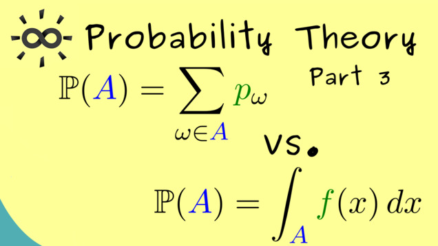
7 00:00:32,186 –> 00:00:36,266 Then in the next step we want to measure the probability of such an event

8 00:00:36,757 –> 00:00:40,800 and this leads us to a general probability measure we call “P”.

9 00:00:41,600 –> 00:00:48,371 Now i can tell you it’s possible to deal with these objects in this abstract sense and then we get a general theory.

10 00:00:48,900 –> 00:00:54,628 However in a lot of applications we find that two special cases are very important here.

11 00:00:55,214 –> 00:00:59,886 So now we distinguish between the discrete case and the continuous case

12 00:01:00,600 –> 00:01:05,400 To be more precise i would also speak of the absolutely continuous case.

13 00:01:06,143 –> 00:01:12,814 Now all the other possibilities we can’t put into these two boxes we will ignore at least for this video.

14 00:01:13,329 –> 00:01:18,671 Indeed often at the start of probability theory one focuses at discrete problems.

15 00:01:19,300 –> 00:01:23,029 They are easy to explain, when we only have finitely many outcomes.

16 00:01:23,743 –> 00:01:29,057 However i would also say that we have a discrete problem when we have infinitely many outcomes

17 00:01:29,257 –> 00:01:32,700 if they still are countable like the natural numbers.

18 00:01:33,471 –> 00:01:41,471 For example we could throw a die infinitely many times and we count how many throws we needed to get the first six

19 00:01:42,057 –> 00:01:46,943 Then we are still in the discrete case, because we can count all the possible outcomes.

20 00:01:47,567 –> 00:01:54,200 On the other hand in the absolutely continuous case we have infinitely many outcomes, but they are uncountable.

21 00:01:54,667 –> 00:01:58,733 The typical example here would be a dart board where you throw a dart.

22 00:01:59,500 –> 00:02:03,083 There all the values in the disk are possible outcomes.

23 00:02:03,533 –> 00:02:09,999 Okay so that’s the rough idea for the two special cases here and now i would say let’s go into the details.

24 00:02:10,950 –> 00:02:16,567 For this let’s do a table such that we can compare the discrete case and the absolutely continuous case.

25 00:02:17,133 –> 00:02:19,617 First let’s start with the sample space omega.

26 00:02:19,650 –> 00:02:23,017 Which is a finite or countable set in the discrete case.

27 00:02:23,500 –> 00:02:27,650 For example if you flip a coin. Omega would be a set with two elements.

28 00:02:28,267 –> 00:02:32,300 Or giving an infinite example. Omega could be the natural numbers.

29 00:02:33,050 –> 00:02:38,150 On the other hand for our continuous case the sample space omega should be an uncountable set.

30 00:02:38,717 –> 00:02:41,983 and usually we can choose it as a subset of “R^n”

31 00:02:43,100 –> 00:02:46,850 To be even more precise omega should be a so called Borel set.

32 00:02:47,833 –> 00:02:51,467 So it’s an element of the Borel sigma algebra of “R^n”.

33 00:02:52,033 –> 00:02:56,717 If you don’t know what the borel sigma algebra is don’t worry. I have a whole video about it.

34 00:02:57,317 –> 00:03:01,617 However at least for the sake of this video it’s not the most important thing to know here.

35 00:03:02,450 –> 00:03:06,233 Just think of a common example. Omega could be the unit interval.

36 00:03:06,900 –> 00:03:09,317 I choose it as closed here, but it could also be open.

37 00:03:10,017 –> 00:03:13,417 Ok, that is what you should know about possible sample spaces.

38 00:03:14,583 –> 00:03:17,650 Then in the next step let’s talk about the sigma algebras.

39 00:03:18,583 –> 00:03:22,883 In the discrete case it’s very simple. You can just take the whole power set of omega.

40 00:03:23,333 –> 00:03:30,200 Of course depending on the problem you could choose a smaller one, but there is no restriction for choosing the largest one, the power set.

41 00:03:30,850 –> 00:03:35,467 Therefore in the discrete case we don’t have to care about the sigma algebra at all.

42 00:03:36,217 –> 00:03:41,683 However we really need the notion of a sigma algebra on the right hand side. In the continuous case.

43 00:03:42,233 –> 00:03:48,533 There in general it’s not possible to choose the power set, but it’s always possible to take the Borel sigma algebra.

44 00:03:49,400 –> 00:03:53,967 This means that we don’t have all the subsets of omega, but still a lot of them.

45 00:03:54,550 –> 00:03:59,267 Therefore our probability measure can still give probabilities to a lot of events.

46 00:03:59,850 –> 00:04:04,517 Speaking of probability measures this is the next thing we want to compare in both cases.

47 00:04:05,183 –> 00:04:10,783 In the discrete case measuring a singleton, so a set with only one element, is very useful,

48 00:04:11,433 –> 00:04:18,750

because if you know these numbers for all lowercase omega in the sample space omega you know the whole probability measure.

49 00:04:19,733 –> 00:04:23,583 This immediately comes out of the sigma additivity of the probability measure.

50 00:04:24,550 –> 00:04:28,667 As a reminder it’s this property here we discussed in the last video.

51 00:04:29,450 –> 00:04:38,117 Now because of this property in the discrete case instead of the probability measure we can equivalently write down a probability mass function.

52 00:04:38,868 –> 00:04:43,750 Usually one uses a lowercase “p” for this and omega is found in the index.

53 00:04:44,417 –> 00:04:50,500 Of course in the end it should have the same meaning as this probability, but now this function is our starting point.

54 00:04:51,200 –> 00:04:54,467 I say function, but usually we write it as a sequence.

55 00:04:54,900 –> 00:04:59,322 Depending on omega the sample space is a finite sequence or a countable one.

56 00:05:00,044 –> 00:05:05,383 Now because we want to use this for probabilities we claim that this number is always non-negative.

57 00:05:06,250 –> 00:05:10,867 and also the series or sum through all omegas should be exactly one.

58 00:05:11,567 –> 00:05:16,899 If we have such a sequence that fulfills these two properties we call it a probability mass function

59 00:05:17,517 –> 00:05:20,500 and with this we can define the probability measure.

60 00:05:21,367 –> 00:05:29,917 For any event “A” we can set P(A) the sum or series over “p_omega” where omega goes through all the elements in “A”.

61 00:05:30,650 –> 00:05:37,383 There you see the big advantage in the discrete case. We just have countably many numbers involved and also only sums.

62 00:05:38,367 –> 00:05:41,100 So each probability can be written as such a sum.

63 00:05:41,817 –> 00:05:45,617 On the other hand that’s is not possible in the absolutely continuous case.

64 00:05:46,133 –> 00:05:49,609 However for a probability measure there we have something similar,

65 00:05:50,500 –> 00:05:56,383 because like in the example with the dartboard the probability of a single point is just zero.

66 00:05:57,083 –> 00:06:01,383 There are just too many points to get a non-zero probability for a single one.

67 00:06:02,217 –> 00:06:05,633 However we can say something about the density of the probabilities

68 00:06:06,450 –> 00:06:12,667 or to put it in other words it’s no problem at all to measure the probability of a whole region instead of a single point.

69 00:06:13,617 –> 00:06:18,767 Now this density function we simply call “f” and it’s defined on the whole sample space omega

70 00:06:19,383 –> 00:06:24,517 and because we want to measure probabilities we have the same two properties as on the left hand side.

71 00:06:25,350 –> 00:06:29,067 The first one is at each point we have a non-negative number

72 00:06:29,533 –> 00:06:35,133 and you see because in this case omega is a subset of “R^n”. We usually use the letter “x”.

73 00:06:36,017 –> 00:06:38,767 but still here “x” is an element of omega.

74 00:06:39,550 –> 00:06:44,633 Ok now for the second property we have to translate this sum into a continuous case.

75 00:06:45,150 –> 00:06:49,900 This means that here we want that the integral of the function “f” is equal to 1.

76 00:06:50,733 –> 00:06:54,167 It’s the integral where we integrate over the whole domain omega.

77 00:06:55,083 –> 00:07:01,400 Please note here in our simple example it would be a one-dimensional integral, but in general we have an n-dimensional integral

78 00:07:02,100 –> 00:07:05,950 but then you see it’s completely similar to the thing we wanted in the discrete case.

79 00:07:06,683 –> 00:07:12,883 Therefore in the same way the probability measure can be defined, P(A) is the integral where we have the domain “A” .

80 00:07:13,950 –> 00:07:17,760 Ok and with this you see this is our translation between both cases.

81 00:07:18,633 –> 00:07:25,533 However to be honest i omitted one technical detail here on the right hand side, because here we have to deal with sigma algebras.

82 00:07:26,150 –> 00:07:30,550 For this reason this density function “f” here needs to be measurable.

83 00:07:31,533 –> 00:07:35,050 It’s a property we need such that all the integrals here make sense.

84 00:07:35,783 –> 00:07:40,217 If you don’t know this term measurable yet, don’t worry we will talk about it later.

85 00:07:41,083 –> 00:07:45,467 At the moment i would say it’s sufficient that you know that we need some technical detail here.

86 00:07:46,233 –> 00:07:51,333 Ok, i think that’s enough for the theory. Lets talk about some practical examples.

87 00:07:52,317 –> 00:07:56,333 In the discrete case let’s look again at the example of throwing one die.

88 00:07:57,100 –> 00:08:00,133 However maybe this time let’s take an unfair die.

89 00:08:00,983 –> 00:08:05,083 This means that we have different probabilities in the probability mass function.

90 00:08:05,683 –> 00:08:10,917 So we can bring different non-negative probabilities in, but they have to sum up to 1.

91 00:08:11,800 –> 00:08:18,950 For example we could set all the numbers one to five to one tenth and then the probability of getting a six would be one half.

92 00:08:19,700 –> 00:08:25,550 So maybe as a test let’s calculate the probability of the event that we don’t get a 6.

93 00:08:26,367 –> 00:08:34,683 Now by definition this would be the sum of omega going from 1 to 5 and there we have our “p_omega”.

94 00:08:35,400 –> 00:08:43,883 Which in our case is exactly 1 over 10 for all omegas involved here and there you see we get out one half as expected.

95 00:08:44,950 –> 00:08:48,450 Ok, then on the other side let’s look at a continuous example.

96 00:08:49,133 –> 00:08:52,633 Ok, maybe let’s take the interval from 0 to 2 here.

97 00:08:53,350 –> 00:08:56,850 So you see our dart board from before is one-dimensional now.

98 00:08:57,533 –> 00:09:00,850 So we randomly throw one point into this interval.

99 00:09:01,567 –> 00:09:05,617 Then the question would be what is now our probability density function “f”?

100 00:09:06,583 –> 00:09:11,817 Now because we want to have an uniform probability here we need to take a constant function

101 00:09:12,483 –> 00:09:17,333 and because we want to fulfill these two properties there is only one reasonable choice.

102 00:09:18,233 –> 00:09:21,150 We take the constant function with value one half.

103 00:09:21,967 –> 00:09:29,167 So maybe let’s check that the integral property is indeed fulfilled. So we have the integral 0 to 2 and f(x) inside.

104 00:09:30,083 –> 00:09:35,583 Now we can pull the constant one half outside and then only the length of the interval here remains.

105 00:09:36,217 –> 00:09:39,100 Which is of course 2 such that we get out 1.

106 00:09:39,917 –> 00:09:45,233 Ok, then maybe the last question here is can you calculate the probability of a subset “A” here?

107 00:09:45,950 –> 00:09:50,967 As we know the probability is defined as the integral where we integrate over the set “A” here.

108 00:09:51,833 –> 00:09:56,883 Doing the same as before. We can pull out the constant and only the simple integral remains.

109 00:09:58,017 –> 00:10:05,667 Now this one is what we call in general the volume of “A” or in this case, because it’s only one-dimensional we could call it the length of “A”.

110 00:10:06,700 –> 00:10:09,842 or we could simply say it’s the lebesgue measure of “A”.

111 00:10:11,383 –> 00:10:16,805 This sounds now more complicated than it really is, because for intervals we can immediately calculate it.

112 00:10:17,633 –> 00:10:24,763 For example if we have the interval [a, b] we can calculate that this is 0.5*(b - a).

113 00:10:25,317 –> 00:10:30,784 So you could say in this example we just calculate lengths, but then we have to normalize it.

114 00:10:31,400 –> 00:10:34,309 Which means we divide by the full length which is 2.

115 00:10:35,133 –> 00:10:37,142 and indeed then we get a probability.

116 00:10:38,083 –> 00:10:43,340 Ok, with this i hope you now know how to distinguish between discrete and continuous cases.

117 00:10:44,250 –> 00:10:48,185 They are indeed the typical examples that occur. Therefore it’s good to know them.

118 00:10:48,800 –> 00:10:52,479 Then in the next videos we will look at more complicated examples.

119 00:10:52,983 –> 00:10:56,333 Therefore i hope i see you there and have a nice day. Bye!

Q1: If $\Omega = \mathbb{N}$, do we have a discrete or continuous case?

A1: Discrete.

A2: Continuous.

A3: Both cases are possible.

Q2: In the discrete case, what is the common choice for the $\sigma$-algebra?

A1: $\mathcal{A} = \Omega$

A2: $\mathcal{A} = { \emptyset, \Omega }$

A3: $\mathcal{A} =\mathcal{P}(\Omega)$

Q3: In the (absolutely) continuous, we have a probability density function $f: \Omega \rightarrow \mathbb{R}$. What is not a property of this function?

A1: $f(x) \geq 0$

A2: $f(x) \leq 1$

A3: $\int_\Omega f(x) , dx = 1$