00:00 Intro

00:10 Binomial distribution

06:27 Binomial distribution in RStudio

09:40 Urn model in RStudio

14:55 Comparison of urn model and rbinom in RStudio

15:36 Endcard

1 00:00:00,250 –> 00:00:03,719 Hello and welcome back to probability theory.

2 00:00:04,263 –> 00:00:09,554 and first, as always i want to thank all the nice people that support this channel on Steady or Paypal.

3 00:00:10,375 –> 00:00:14,063 Now in todays part 4 we will talk about the binomial distribution.

4 00:00:14,775 –> 00:00:18,886 It’s a fundamental probability measure which occurs a lot in discrete models.

5 00:00:19,800 –> 00:00:22,486 For example we have it when we flip a coin.

6 00:00:22,938 –> 00:00:27,241 Then we would say we only have two possible outcomes. Heads or tails.

7 00:00:27,829 –> 00:00:34,239 Now if we don’t have fair coin, but a bias coin. We use the letter “p” for the probability of heads.

8 00:00:34,629 –> 00:00:40,001 For the sake of this video lets assume that “p” is a rational number between 0 and 1.

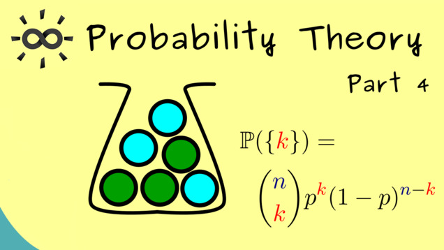
9 00:00:40,886 –> 00:00:44,971 This makes everything simpler, because we can write “p” as a fraction.

10 00:00:45,314 –> 00:00:48,786 For example we could write it as “a” divided by “a + b”.

11 00:00:49,443 –> 00:00:53,286 Of course here “a” and “b” are natural numbers including 0.

12 00:00:53,871 –> 00:00:59,572 For example if we have a fair coin, so a normal coin, the probability “p” should be 0.5.

13 00:01:00,157 –> 00:01:03,547 This means that we can choose both “a” and “b” to be 1.

14 00:01:04,214 –> 00:01:08,714 If we have this we can see the whole random experiment in a different light.

15 00:01:09,144 –> 00:01:13,122 More concretely this is what we usually call an urn model.

16 00:01:13,943 –> 00:01:18,557 Now such an urn is just a container, were we can put in different kind of balls.

17 00:01:19,128 –> 00:01:24,100 In our case here we take green balls for heads and red balls for tails.

18 00:01:24,520 –> 00:01:28,379 Indeed the number of balls should be “a” in the case of heads

19 00:01:28,579 –> 00:01:30,400 and “b” in the case of tails.

20 00:01:31,014 –> 00:01:36,616 Hence here our random experiment is that one ball is drawn randomly from the jar.

21 00:01:36,971 –> 00:01:41,657 and then the probability for getting a green heads ball is again our “p”.

22 00:01:42,029 –> 00:01:47,429 It’s simply the ratio of the number of green balls to the number of all balls in the urn.

23 00:01:47,943 –> 00:01:51,886 Therefore in both cases we have the same probability measure.

24 00:01:52,371 –> 00:01:56,398 Here the sample space Omega is simply the set with two elements.

25 00:01:56,957 –> 00:02:01,729 We call them “H” and “T” in this case, but of course the names are not so important here.

26 00:02:02,229 –> 00:02:05,706 Often you also see 0 and 1 for the two elements.

27 00:02:05,986 –> 00:02:12,681 Here we have a discrete case. Therefore the probability measure can be defined with a probability mass function.

28 00:02:13,371 –> 00:02:18,221 Or in other words we just have to say what is the probability for the single outcomes.

29 00:02:18,643 –> 00:02:24,410 For heads we have “a” divided by “a + b” and for tails we have “b” divided by “a + b”.

30 00:02:24,700 –> 00:02:28,055 and then you see they add up to 1, as they should.

31 00:02:28,586 –> 00:02:34,815 Therefore usually we just call the one probability here “p” and the other one “1 - p”.

32 00:02:35,071 –> 00:02:40,414 Ok, by knowing all this we now can start talking about the binomial distribution.

33 00:02:41,043 –> 00:02:45,105 Here we don’t have a single coin toss, but now we do it n-times.

34 00:02:45,700 –> 00:02:49,331 Hence after n tosses we just count the number of heads.

35 00:02:49,814 –> 00:02:54,231 and importantly we are not interested in which order heads and tails occurred.

36 00:02:54,700 –> 00:02:59,569 Now you already know equivalently we could also describe this with n urns.

37 00:03:00,200 –> 00:03:05,049 We just draw one ball from each urn and then we count the heads as well.

38 00:03:05,343 –> 00:03:10,347 Of course this would be a little bit wasteful, because we don’t need so many urns for this.

39 00:03:10,571 –> 00:03:15,040 We just take one urn and then we draw n balls with replacement.

40 00:03:15,614 –> 00:03:20,922 This means that we draw the first ball, note it and then we put the ball back into the jar.

41 00:03:21,222 –> 00:03:26,361 Therefore for the second draw we still have the same ratio of balls inside the urn.

42 00:03:26,814 –> 00:03:31,479 So in summary there are 3 things for the binomial distribution you should remember.

43 00:03:32,014 –> 00:03:33,757 The sample size is “n”.

44 00:03:33,814 –> 00:03:36,289 It’s unordered and with replacement.

45 00:03:36,786 –> 00:03:42,596 Now because we are just interested in the number of heads, you already know the corresponding sample space.

46 00:03:43,414 –> 00:03:46,959 The minimal case would be that we only have 0 heads.

47 00:03:47,159 –> 00:03:49,949 and then of course the maximum would be “n”.

48 00:03:50,529 –> 00:03:53,114 Now as before this is a discrete model.

49 00:03:53,257 –> 00:03:57,369 Hence the probability measure can be given with a probability mass function.

50 00:03:57,843 –> 00:04:01,925 So it’s sufficient to define what the probability of “k” heads is.

51 00:04:02,425 –> 00:04:06,940 Ok, maybe i first give you the definition and then we talk about why this makes sense.

52 00:04:07,471 –> 00:04:10,086 So here we have the binomial “n choose k”.

53 00:04:10,529 –> 00:04:15,169 Then we have “p” to power “k” times (1 - p) to the power (n - k).

54 00:04:15,829 –> 00:04:20,500 Now what you should see immediately is that for the binomial distribution we have exactly two parameters.

55 00:04:21,043 –> 00:04:23,114 The size “n” and the probability “p”.

56 00:04:23,971 –> 00:04:27,642 Now please recall “p” was the probability for just one coin toss.

57 00:04:28,286 –> 00:04:32,317 and with this knowledge we now can explain this formula here.

58 00:04:32,517 –> 00:04:36,117 Ok lets visualize all the coin tosses with a tree.

59 00:04:36,317 –> 00:04:42,277 So for the first coin toss we have the probability “p” to get heads and “1 - p” to get tails.

60 00:04:42,800 –> 00:04:46,595 and then of course we get the same picture for the second coin toss.

61 00:04:46,795 –> 00:04:51,099 Of course this then just repeats until we reach the n-th level.

62 00:04:51,686 –> 00:04:58,942 Ok, now for the probability “P({k})” here, we need to go through all the possibilities, where we hit exactly “k” heads.

63 00:04:59,600 –> 00:05:03,157 For example if we want to hit 2 heads we can go through here,

64 00:05:03,186 –> 00:05:08,329 Then we hit this one. Then we go to this one, but then we have to hit tails.

65 00:05:08,800 –> 00:05:14,331 Therefore for the probability of this route we have “p” times “p” times “1 - p”

66 00:05:14,929 –> 00:05:18,800 In other words the power of “p” gives us the number of heads we hit

67 00:05:19,000 –> 00:05:23,157 and the power for “1 - p” gives us the number of tails we hit.

68 00:05:23,651 –> 00:05:27,971 However you already see there are more possibilities to hit exactly 2 heads.

69 00:05:28,729 –> 00:05:34,465 For example this route here gives out exactly 2 heads with the same probability as this one.

70 00:05:34,665 –> 00:05:37,690 Also on the right hand side we find this route here.

71 00:05:38,429 –> 00:05:43,587 Hence we have to multiply the probability here with 3 or with “3 choose 2”.

72 00:05:44,171 –> 00:05:50,767 In fact it’s a very good exercise to show that the number of possible ways is exactly given by “n choose k”.

73 00:05:51,457 –> 00:05:58,334 In summary this picture now explains why the definition of the probability measure for the binomial distribution makes sense.

74 00:05:58,971 –> 00:06:04,229 Also i can tell you there are a lot of different notations you can find for this probability measure.

75 00:06:04,795 –> 00:06:09,326 For example some people write “B” with the 2 parameters “n” and “p”.

76 00:06:09,999 –> 00:06:13,837 also a lot little bit longer you would also find “Bin”.

77 00:06:14,329 –> 00:06:22,015 However no matter which notation is used you always should know what is the definition of the mass function and what is the meaning of “n” and “p”.

78 00:06:22,729 –> 00:06:26,657 If you forget it maybe our programming language “R” can help you.

79 00:06:26,943 –> 00:06:30,129 Therefore in the next step lets open RStudio.

80 00:06:30,743 –> 00:06:33,416 So here you see the nice 4 windows again.

81 00:06:34,471 –> 00:06:39,702 and we can immediately go to console and ask “R” about the binomial distribution.

82 00:06:40,257 –> 00:06:46,810 Therefore we type ?rbinom, enter and here we see the help function.

83 00:06:47,010 –> 00:06:49,871 It tells you a little bit about the binomial distribution.

84 00:06:50,044 –> 00:06:55,512 For example its interpretation and also shows you some commands to use it in “R”.

85 00:06:56,143 –> 00:07:01,715 We will just use the rbinom command here, were the arguments are explained afterwards.

86 00:07:02,514 –> 00:07:09,729 Most importantly you should check that size is really our “n” from before and this prob is our “p” from before.

87 00:07:10,786 –> 00:07:13,151 Of course this is what you will find here.

88 00:07:13,914 –> 00:07:18,856 So you see number of trials and probability of success on each trial.

89 00:07:19,743 –> 00:07:25,692 Now if we go further you also see that the probability mass function is also included here.

90 00:07:26,057 –> 00:07:29,840 and there you see they also use “n” and “p” as we did.

91 00:07:30,529 –> 00:07:35,361 The only difference is that they use letter “x” where we used the letter “k” before.

92 00:07:36,157 –> 00:07:42,523 Ok with this you should see it’s very nice that we have the manual of probability theory included in “R”

93 00:07:43,271 –> 00:07:46,300 Ok then lets use the command as we had it in the picture

94 00:07:47,043 –> 00:07:53,447 So lets type rbinom, 1, then the size 3 and maybe the probability 0.5.

95 00:07:54,571 –> 00:07:57,971 Now this means we do the random experiment and get a number of heads.

96 00:07:58,990 –> 00:08:02,328 So you see in this case we only got one head.

97 00:08:02,786 –> 00:08:05,207 Therefore i would say lets do it again.

98 00:08:06,286 –> 00:08:09,795 Now we got 2 heads corresponding to our picture from before.

99 00:08:10,586 –> 00:08:14,959 Of course we can do it again and again and maybe we get different results.

100 00:08:15,386 –> 00:08:21,084 Now here 0 would be the lowest number that can come out and 3 would be the largest one.

101 00:08:22,086 –> 00:08:25,636 Ok at this point we can talk about this number 1 here.

102 00:08:26,429 –> 00:08:31,168 Indeed what we did manually before we can tell “R” with this number.

103 00:08:31,368 –> 00:08:35,950 So you see when i put in 10 we get out 10 results.

104 00:08:37,000 –> 00:08:41,115 So we tell “R” please repeat the random experiment 10 times.

105 00:08:41,315 –> 00:08:47,580 So you see without much work. Without flipping all the coins we immediately get all the results we want.

106 00:08:47,943 –> 00:08:51,922 For example if you want 100 that’s no problem at all.

107 00:08:52,814 –> 00:08:56,999 Now if you want to visualize this we can use the histogram command.

108 00:08:57,329 –> 00:09:01,664 So lets simply put the rbinom command into the histogram command.

109 00:09:02,714 –> 00:09:05,871 and then we get immediately this nice picture

110 00:09:06,629 –> 00:09:11,637 Obviously since we only have 4 possible outcomes, we don’t see so much here.

111 00:09:11,837 –> 00:09:16,725 However we already see that 0 or 3 as an outcome is very unlikely.

112 00:09:17,757 –> 00:09:22,843 Therefore maybe we can look what happens when we increase the size of our random experiment.

113 00:09:23,414 –> 00:09:26,543 So this is our “n” in the formula. So we flip more coins.

114 00:09:27,029 –> 00:09:29,103 So lets increase it to 30.

115 00:09:29,471 –> 00:09:32,423 Then we hit enter and you see the new histogram.

116 00:09:33,371 –> 00:09:38,936 also here we see the outcomes in the middle are much more probable then the outcomes in the extrema.

117 00:09:39,743 –> 00:09:44,329 Ok, then for our next step i would say lets put our urn into “R”.

118 00:09:44,686 –> 00:09:47,860 Here please remember we had 2 numbers for our urn.

119 00:09:48,614 –> 00:09:52,752 a number “a” and the number “b” for heads and tails respectively.

120 00:09:53,300 –> 00:09:56,368 So lets try to put that into RStudio.

121 00:09:56,829 –> 00:09:59,609 For this lets use the script in the top left corner.

122 00:10:00,486 –> 00:10:03,070 Hence lets choose a number for “a”. For example 5.

123 00:10:03,270 –> 00:10:05,978 and lets add comment with the number sign.

124 00:10:06,486 –> 00:10:09,732 So for us this is the number of heads in the urn.

125 00:10:09,932 –> 00:10:14,197 Then lets do the same with the number “b”. For example lets choose 7.

126 00:10:14,614 –> 00:10:17,884 and then number of tails in the urn.

127 00:10:18,671 –> 00:10:24,114 Now, because it’s easier to calculate with numbers lets say that heads is represented by ones.

128 00:10:24,457 –> 00:10:26,487 and tails represented by zeros.

129 00:10:26,900 –> 00:10:32,370 Ok now i can tell you if you push control, Alt and “r”, we run the whole script.

130 00:10:32,886 –> 00:10:36,996 So you see everything here is in the console and the values are saved.

131 00:10:37,386 –> 00:10:41,521 Ok, now you know we want to define an urn with zeros and ones.

132 00:10:42,014 –> 00:10:46,186 You already know we can put numbers together with the c command here.

133 00:10:46,443 –> 00:10:52,343 In this case you see we have an urn, where we have the 1-ball onces and the 0-ball also once.

134 00:10:52,871 –> 00:10:56,640 Of course that is not what we want. We want more balls in it.

135 00:10:57,214 –> 00:10:59,681 Then we would have to type something like this.

136 00:10:59,943 –> 00:11:04,007 Here you can see we have 12 balls in it, with the correct ratio.

137 00:11:04,657 –> 00:11:11,078 Obviously this is not what we want to do, because then we can’t change the numbers “a” and “b” here at the beginning.

138 00:11:11,529 –> 00:11:14,214 Indeed we will use the replicate command.

139 00:11:14,671 –> 00:11:17,727 So we write urn = rep,

140 00:11:17,927 –> 00:11:23,351 then we put in the different kinds of balls we want. So in this case 1 and 0.

141 00:11:23,971 –> 00:11:27,821 Then a comma and then how many of them we want.

142 00:11:28,021 –> 00:11:30,471 So in this case simply “a” and “b”.

143 00:11:30,886 –> 00:11:33,485 So lets run the script and see what happens.

144 00:11:34,271 –> 00:11:38,747 and there you see this is exactly the urn from before. The urn we wanted.

145 00:11:38,947 –> 00:11:43,386 and of course you can check, if we change the numbers here, the urn will change as well.

146 00:11:44,214 –> 00:11:49,068 Ok, then lets go back to the command window and take a sample from the urn.

147 00:11:49,614 –> 00:11:52,350 So with this command we take one ball out.

148 00:11:52,729 –> 00:11:55,846 Now this was 1, but of course we can repeat it.

149 00:11:56,229 –> 00:12:01,536 Ok, so that’s very nice. It’s working, but maybe now lets take 10 balls out of the urn.

150 00:12:02,071 –> 00:12:05,100 Ok there you see, this is now our sample.

151 00:12:05,786 –> 00:12:09,526 Maybe lets do it again and you see we can do it again and again.

152 00:12:10,786 –> 00:12:13,977 and there you should see the number of 1 is always 3.

153 00:12:14,514 –> 00:12:17,153 However that’s not what we want here in our example,

154 00:12:17,353 –> 00:12:22,474 because it means we take balls out of the urn, but without replacement.

155 00:12:22,786 –> 00:12:29,186 You can check that here, because it would mean the urn would be empty after 10 balls, so 11 won’t work.

156 00:12:29,686 –> 00:12:32,249 and indeed this is what “R” tells us.

157 00:12:33,100 –> 00:12:37,258 Hence the solution is that we have to add the replacement argument here.

158 00:12:37,886 –> 00:12:40,729 So we would write replace = TRUE.

159 00:12:41,300 –> 00:12:45,179 Ok, so lets check what comes out as a sample as we want it.

160 00:12:45,543 –> 00:12:48,614 So maybe lets do it again to check how many ones we can have.

161 00:12:49,629 –> 00:12:52,044 Ok, at this point you should see, it’s working.

162 00:12:52,557 –> 00:12:55,043 So now please recall our random experiment.

163 00:12:55,400 –> 00:13:00,376 We are not interested in the overall order here, but only how many 1 we got.

164 00:13:00,743 –> 00:13:05,605 Therefore the natural question would be how can we count them easily in “R”?

165 00:13:06,114 –> 00:13:12,055 Now maybe you already see it. We can count the 1, if we just sum up all the numbers involved here.

166 00:13:12,800 –> 00:13:16,300 and the correct command in “R” for this is simply “sum”.

167 00:13:17,157 –> 00:13:20,672 So lets put the sample inside and lets see what comes out.

168 00:13:20,872 –> 00:13:23,476 In this case it’s 0, so lets do it again.

169 00:13:24,086 –> 00:13:26,363 So we see it’s working like a charm.

170 00:13:26,563 –> 00:13:32,181 So i would say lets copy that in our script here, but lets replace 11 with “n”.

171 00:13:32,786 –> 00:13:36,760 Then this “n” is indeed the same, we had in our binomial distribution.

172 00:13:37,571 –> 00:13:42,545 With this our script is working, because each time we run it, we get a number of heads out.

173 00:13:43,414 –> 00:13:47,568 and as before we can do it again and again to get different numbers out.

174 00:13:48,214 –> 00:13:53,807 Therefore maybe for you a natural question would be can we repeat the experiment “m” times.

175 00:13:54,114 –> 00:13:57,005 Maybe the case that m=1000.

176 00:13:57,957 –> 00:14:02,543 and of course also in this case “R” comes with a nice replicate function.

177 00:14:02,986 –> 00:14:11,315 We just put the command “replicate” in front of the thing we want to replicate and before we put the number of times we want to replicate it.

178 00:14:11,543 –> 00:14:14,674 So simply close the parentheses and then we are finished.

179 00:14:15,329 –> 00:14:17,559 So lets run it to see what comes out.

180 00:14:18,671 –> 00:14:22,948 and there you see we have 1000 numbers for our random experiment.

181 00:14:23,814 –> 00:14:27,937 Now to make our life a little bit easier lets give this list a name.

182 00:14:28,137 –> 00:14:30,461 So lets call it observations.

183 00:14:31,743 –> 00:14:36,631 and then in the next step i would say lets visualize this list in a histogram.

184 00:14:37,214 –> 00:14:39,871 and this command you already know. It’s just “hist”.

185 00:14:40,443 –> 00:14:44,879 Ok, when we run the script now we should see the histogram of observations.

186 00:14:45,657 –> 00:14:48,977 Maybe lets run it again to see how much changes.

187 00:14:49,786 –> 00:14:54,826 Now by using these 2 arrows here you can see, we don’t have so many differences at all.

188 00:14:55,914 –> 00:15:02,200 For the end now, the last question we can answer is, how does this compare to the binomial distribution in “R”?

189 00:15:02,629 –> 00:15:05,757 So lets do the histogram of rbinom.

190 00:15:06,471 –> 00:15:11,013 and here we have to put in “m , n” and then “p”.

191 00:15:11,100 –> 00:15:15,029 and here in our case “p” is 3 divided by 10.

192 00:15:15,471 –> 00:15:20,129 So lets put that in here and then lets see what the histogram looks like.

193 00:15:20,971 –> 00:15:24,166 Indeed we see, we have a similar distribution.

194 00:15:24,657 –> 00:15:29,758 Of course this is what we expected after this long video about the binomial distribution.

195 00:15:30,500 –> 00:15:34,273 So with this i think it’s enough for today. See you in the next video.

196 00:15:35,000 –> 00:15:36,675 Have a nice day. Bye!

Q1: What is the sample space for the binomial distribution $\mathrm{Bin}(n,p)$?

A1: $\Omega = \mathbb{N}$

A2: $\Omega = {1,2, \ldots, n } $

A3: $\Omega = {0,1,2, \ldots, n } $

A4: $\Omega = {1,2, \ldots, n-1 } $

Q2: What is the probability mass function of the binomial distribution $\mathrm{Bin}(n,p)$?

A1: $\mathbb{P}({ k } ) = \binom{n}{k} p^k (1-p)^{-k}$

A2: $\mathbb{P}({ k } ) = \binom{n}{k} p^k (1-p)^{n-k}$

A3: $\mathbb{P}({ k } ) = \binom{n}{k} p^k (1-p)^{n}$

Q3: What is a possible outcome of the following R code? $$\texttt{urn = c(1,0,0)}$$ $$\texttt{replicate(3,sum(sample(urn,10,replace=TRUE)))}$$

A1: $\texttt{5, 3, 4}$

A2: $\texttt{1, 2}$

A3: $\texttt{11, 40, 2}$

A4: $\texttt{11, 4, 2, 3}$

A5: $\texttt{3, 3, 3, 3}$