00:00 Intro

00:13 Hypergeometric distriubution

02:21 Writing a sample space for Hypergeometric function

05:42 Hypergeometric distribution for 2 colours

07:06 Hypergeometric distribution in R

10:29 Outro

1 00:00:00,400 –> 00:00:03,514 Hello and welcome back to probability theory.

2 00:00:04,129 –> 00:00:08,896 and as always first i want to thank all the nice people that support this channel on Steady or Paypal.

3 00:00:09,471 –> 00:00:13,562 Now in todays part 6 we will talk about the Hypergeometric distribution.

4 00:00:13,943 –> 00:00:18,350 It’s the name for an important probability measure, we find for discrete cases.

5 00:00:18,771 –> 00:00:25,230 and here we will talk about the general formulation for it. Also called the multivariant Hypergeometric distribution.

6 00:00:25,714 –> 00:00:29,384 Here you can immediately keep 3 important ingredients in mind.

7 00:00:29,584 –> 00:00:32,500 First the size is given by a natural number n,

8 00:00:32,686 –> 00:00:35,804 The sample is unordered and without replacement.

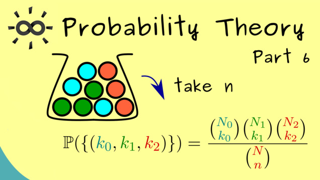
9 00:00:36,557 –> 00:00:40,203 Hence a useful visualisation is again given by an urn model.

10 00:00:40,829 –> 00:00:46,383 This means that in this model we take out n balls from the urn and look what we get.

11 00:00:46,583 –> 00:00:49,925 So we don’t have an order and we don’t replace the balls.

12 00:00:50,125 –> 00:00:53,659 Therefore in short you could say we draw n balls at once.

13 00:00:53,859 –> 00:00:59,054 and there you should see, this is only interesting if we have different coloured balls in the urn.

14 00:00:59,671 –> 00:01:02,486 For example we could have 4 different colours here.

15 00:01:03,043 –> 00:01:07,871 Hence our first question here is: how can we mathematically formulate this?

16 00:01:08,329 –> 00:01:13,682 First we can say that the different colours are just given by a finite set we call capital C.

17 00:01:14,343 –> 00:01:19,961 In our example here we could just index the colours, so we choose numbers from 0 to 3.

18 00:01:20,161 –> 00:01:25,951 Of course every set with 4 elements would do the work, but working with numbers is much easier for calculations.

19 00:01:26,857 –> 00:01:34,509 Also here in our simple example we could talk about possible outcomes, maybe in the case that n is equal to 5.

20 00:01:34,786 –> 00:01:41,336 One possible sample could be this one, where we have 2 green balls, 1 red ball, 1 blue ball and 1 orange ball.

21 00:01:41,943 –> 00:01:46,051 We don’t have an order. We can just count how many balls of each colour we have.

22 00:01:46,743 –> 00:01:54,346 Hence in mathematical terms, here we would have a function from the set of colours, C into the natural numbers including 0.

23 00:01:55,014 –> 00:01:59,834 and there you see immediately it’s very helpful to index the colours with numbers.

24 00:02:00,414 –> 00:02:05,124 Because then we can rewrite this function into a tuple with 4 coordinates.

25 00:02:05,686 –> 00:02:11,542 So in this example here we would have 2 green balls, 1 red one, 1 blue one and 1 orange one.

26 00:02:12,029 –> 00:02:16,893 So what we always should have is that the sum of all these numbers is equal to 5.

27 00:02:17,329 –> 00:02:21,489 Then this could be a possible outcome of our random experiment here.

28 00:02:21,689 –> 00:02:26,387 Ok now with this knowledge we are able to write down the sample space Omega.

29 00:02:26,587 –> 00:02:30,530 It’s simple the set of all functions or tuples of this form.

30 00:02:31,171 –> 00:02:37,607 So in general we would say, we have numbers k_c, where the lower case c goes through all the colours in set C.

31 00:02:38,171 –> 00:02:43,269 and then we say, this is an element of the natural numbers including 0 to the power c.

32 00:02:43,469 –> 00:02:49,174 So this is the general notation of all the functions from the set C into N_0.

33 00:02:49,800 –> 00:02:55,691 It’s a helpful notation, because it reminds us that we can also rewrite the function as a tuple.

34 00:02:55,891 –> 00:02:58,890 and we also put that into this notation here.

35 00:02:59,400 –> 00:03:04,243 Ok and now the only condition we have here is that all these numbers add up to n.

36 00:03:04,600 –> 00:03:08,679 So we can simply write: sum of k_c is equal to n.

37 00:03:08,879 –> 00:03:11,673 and then we have our whole sample space Omega.

38 00:03:12,243 –> 00:03:19,177 Of course you already know as for all discrete cases the sigma algebra is just chosen as just the power set of Omega.

39 00:03:19,414 –> 00:03:22,923 Therefore we can immediately go to the probability measure.

40 00:03:23,123 –> 00:03:27,749 and maybe also for this it’s helpful to first look at our example here.

41 00:03:28,243 –> 00:03:32,009 For our example you already know we have tuples of 4 elements.

42 00:03:32,357 –> 00:03:38,126 Hence we can say we have k_0, k_1, k_2, k_3 from N_0 to the power 4.

43 00:03:38,326 –> 00:03:41,796 and also the sum should be the sample size n.

44 00:03:41,996 –> 00:03:46,571 Now you might already see for calculating the probability of an outcome,

45 00:03:46,657 –> 00:03:50,786 we have to know how many balls of each colour are actually in the urn.

46 00:03:51,114 –> 00:03:53,929 For this we have to introduce new variables.

47 00:03:54,327 –> 00:03:58,448 Hence capital N with index c stands for this number.

48 00:03:58,648 –> 00:04:04,155 and then of course the total number of balls in the urn is given by the sum of all these numbers.

49 00:04:05,014 –> 00:04:08,293 Here we will simply use the symbol N for it.

50 00:04:08,493 –> 00:04:12,713 Ok, now by knowing all this we can start calculating probabilities.

51 00:04:13,386 –> 00:04:18,538 As always in discrete cases knowing the probability mass function is enough.

52 00:04:18,738 –> 00:04:22,143 Hence we just calculate the probability of a singleton.

53 00:04:22,871 –> 00:04:26,154 Now here we just have to count all the possibilities we can have.

54 00:04:26,900 –> 00:04:29,401 and then we will have a fraction here.

55 00:04:30,071 –> 00:04:32,357 Ok, we already know what is in the denominator,

56 00:04:32,454 –> 00:04:37,826 because there we find all possibilities to take n balls from capital N ones.

57 00:04:38,357 –> 00:04:41,543 So we simply have capital N choose lower case n.

58 00:04:42,114 –> 00:04:47,471 Ok, then for the next step, you should see we want exactly k_0 green balls.

59 00:04:47,971 –> 00:04:51,162 So we simply have N_0 choose k_0.

60 00:04:52,000 –> 00:04:55,304 and of course we have the same thing for all the other colours.

61 00:04:55,771 –> 00:04:59,980 Therefore in the next step we have times N_1 choose k_1.

62 00:05:00,529 –> 00:05:05,710 and then times N_2 choose k_2 times N_3 choose k_3.

63 00:05:06,143 –> 00:05:10,678 and with this we have our probability we call the hypergeometric distribution.

64 00:05:11,414 –> 00:05:15,192 Therefore in the next step lets formulate this in a general case.

65 00:05:15,392 –> 00:05:20,514 Also here we just give the probability mass function. So we put in a singleton.

66 00:05:20,714 –> 00:05:23,746 Which we describe as before as k_c.

67 00:05:23,946 –> 00:05:29,976 Then now you know we find a fraction, where in the numerator we find a product of all the colours.

68 00:05:30,357 –> 00:05:33,973 So we have the product symbol with N_c choose k_c.

69 00:05:34,173 –> 00:05:36,860 and the denominator we already know.

70 00:05:37,060 –> 00:05:42,110 Ok and there we have it. This is the hypergeometric distribution in the general case.

71 00:05:42,657 –> 00:05:48,307 Now often only 2 colours are involved, which means the whole thing here gets very simple.

72 00:05:48,771 –> 00:05:53,999 However the simple case is also often known as the hypergeometric distribution.

73 00:05:54,543 –> 00:05:59,542 Therefore it might be worth it to write down the formulas for the special case as well.

74 00:05:59,743 –> 00:06:04,521 Of course the whole set up is the same, but we can make the sample space much simpler.

75 00:06:04,721 –> 00:06:09,772 The reason for that is that for two colours only one degree of freedom remains.

76 00:06:09,972 –> 00:06:15,814 For example if we draw n balls and we count the number of red balls, which means the number of ones

77 00:06:15,986 –> 00:06:19,771 We immediately get the number of green balls, which means the number of zeros.

78 00:06:20,486 –> 00:06:25,157 Hence if we just count the ones, we can say a sample is just the number.

79 00:06:25,357 –> 00:06:30,060 This means that we can take the sample space Omega as a set 0 to n.

80 00:06:30,260 –> 00:06:34,643 and then of course we can also simplify the probability mass function here.

81 00:06:35,129 –> 00:06:39,811 So lets look at P of the singleton k and copy what we already know.

82 00:06:40,011 –> 00:06:42,724 Which means we have N choose n in the denominator

83 00:06:42,924 –> 00:06:45,581 and in the numerator we have 2 factors.

84 00:06:46,014 –> 00:06:51,371 Now here k_1 is simply our k and k_0 is (n-k).

85 00:06:51,758 –> 00:06:58,612 and also we don’t have to write capital N_0 here, because we can use capital N - capital N_1.

86 00:06:58,986 –> 00:07:05,757 and there we have it. This is the compact formulation for the hypergeometric distribution when we only have two kinds of balls.

87 00:07:06,500 –> 00:07:11,944 Now for the last part of this video let me show you, how you can find this distribution in R.

88 00:07:12,571 –> 00:07:16,318 It’s simply given by “rhyper”. So lets look at the manual here.

89 00:07:17,343 –> 00:07:24,900 So you see this is the hypergeometric distribution and if we scroll down you see rhyper and all the variables here.

90 00:07:25,429 –> 00:07:31,011 The arguments are explained below and this k here is actually our lower case n.

91 00:07:31,211 –> 00:07:36,567 and you also see the other variables stand for the number of white balls and the number of black balls.

92 00:07:37,329 –> 00:07:41,755 So in our formulation this would be capital N_1 and capital N_0.

93 00:07:42,357 –> 00:07:46,257 and additionally we have the first argument for the number of repetitions.

94 00:07:46,871 –> 00:07:54,671 Therefore i would say lets see what happens when we have one observation, 9 white balls, 3 black balls and we pull 5 balls out.

95 00:07:55,011 –> 00:07:57,817 Then when we hit enter, we see our outcome.

96 00:07:58,017 –> 00:08:01,318 So the number of white balls we got is just counted.

97 00:08:01,518 –> 00:08:04,772 Ok, then lets repeat the whole random experiment.

98 00:08:05,443 –> 00:08:09,916 So here we got 3 white balls. Which means we got also 2 black ones.

99 00:08:10,586 –> 00:08:16,162 Ok so now maybe we can use the first argument to do a lot of repetitions of this random experiment.

100 00:08:17,071 –> 00:08:18,829 So lets say we do 20.

101 00:08:19,943 –> 00:08:23,433 So there you see we have a lot of of fours, but not a two.

102 00:08:23,957 –> 00:08:26,776 However we know that two is possible.

103 00:08:26,976 –> 00:08:30,023 Therefore maybe lets go to 200 observations.

104 00:08:32,471 –> 00:08:36,495 and there you see, we find some twos, but they are very unlikely.

105 00:08:37,043 –> 00:08:40,091 Hence to visualize that, lets put it into a histogram.

106 00:08:40,291 –> 00:08:42,371 So we put “hist” in front.

107 00:08:42,916 –> 00:08:45,637 and close the parentheses and hit enter.

108 00:08:46,543 –> 00:08:50,358 The first thing we note is that it’s not the best visualization for a histogram yet,

109 00:08:50,558 –> 00:08:53,881 but we already have that two is very unlikely.

110 00:08:54,286 –> 00:09:00,186 Now one possibility to make the whole histogram nicer, is to tell R where it should put the bits.

111 00:09:00,500 –> 00:09:03,514 and these break points we can put into a vector x.

112 00:09:04,329 –> 00:09:09,788 So lets choose steps of one, where we start at 1.5 and end at 5.5.

113 00:09:10,057 –> 00:09:13,029 So lets hit enter and there you see our x.

114 00:09:13,457 –> 00:09:18,607 and this vector x is now what we can put into the histogram function as an argument.

115 00:09:18,807 –> 00:09:25,498 This is not so complicated. We choose the histogram function and then we put in “, " and “breaks”

116 00:09:26,171 –> 00:09:29,522 and then these breaks should be equal to our vector x.

117 00:09:30,214 –> 00:09:33,173 and there you can see, this is what comes out.

118 00:09:33,373 –> 00:09:36,795 So maybe lets repeat it to see immediately what can change.

119 00:09:37,600 –> 00:09:43,769 So it’s almost the same. We have the same behaviour. 2 is very unlikely, but 5 is more likely.

120 00:09:44,486 –> 00:09:48,570 Hence maybe we need to be more precise. Lets go to 2000 repetitions.

121 00:09:48,929 –> 00:09:51,310 and there we get this histogram.

122 00:09:51,929 –> 00:09:56,154 and then i want to repeat it again and again. To see that we are very much stable here.

123 00:09:56,971 –> 00:10:02,154 So what you should see here is, that for this example the highest probability is at 4.

124 00:10:02,354 –> 00:10:05,990 and the lowest is at 2. So we don’t have a symmetric distribution.

125 00:10:06,686 –> 00:10:14,159 This is the case, because we take out a lot of balls compared to the number of balls of each kind inside the urn.

126 00:10:14,359 –> 00:10:17,486 Therefore i would suggest, play around with these numbers

127 00:10:17,487 –> 00:10:21,743 and compare the result with the binomial distribution, we have already discussed.

128 00:10:22,186 –> 00:10:26,555 Ok, then i think it’s good enough for today and i hope i see you in the next video.

129 00:10:27,043 –> 00:10:28,843 Have a nice day. Bye!

Q1: What is the sample space for the hypergeometric distribution where three colours are involved and $n$ balls are drawn from the urn?

A1: $\Omega = \mathbb{N}$

A2: $\Omega = {0,1,2, \ldots, n } $

A3: $\Omega = { (k_1, k_2, k_3) \in \mathbb{N}_0^3 \mid k_0 + k_1 + k_2 = n } $

Q2: What is the probability mass function of the hypergeometric distribution where three colours are involved and $n$ balls are drawn from the urn? Here $N_i$ stands for the number of balls of colour $i$ in the urn and $N$ stands for the total number of balls in the urn.

A1: $\displaystyle \mathbb{P}({ (k_0, k_1, k_2) } ) = \frac{ \binom{ N_0 }{k_0} \binom{ N_1 }{k_1} \binom{ N_2 }{k_2}}{ \binom{N}{n}}$

A2: $\displaystyle \mathbb{P}({ (k_0, k_1, k_2) } ) = \frac{ \binom{ N_0 }{k_0} \binom{ N_1 }{k_1} \binom{ N_2 }{k_2}}{ \binom{n}{N}}$

A3: $\displaystyle \mathbb{P}({ (k_0, k_1, k_2) } ) = \frac{\binom{N}{n} }{\binom{ N_0 }{k_0} \binom{ N_1 }{k_1} \binom{ N_2 }{k_2} }$

Q3: What is a possible outcome of the following R code? $$\texttt{urn = c(1,1,1,1,0,0)}$$ $$\texttt{replicate(3,sum(sample(urn,5,replace=FALSE)))}$$

A1: $\texttt{5, 3, 4}$

A2: $\texttt{1, 2}$

A3: $\texttt{11, 40, 2}$

A4: $\texttt{4, 3, 3}$

A5: $\texttt{3, 3, 3, 3}$

Q4: A team consists of 10 people of three different groups, where 3 are from group A, 2 from group B and 5 from group C. We want to choose a subteam of 3 people by drawing lots. What is the probability of obtaining exactly one person from each group?

A1: $\displaystyle \mathbb{P}({ (3, 2, 5) } ) = \frac{ \binom{ 3 }{3} \binom{ 2 }{2} \binom{ 5 }{5}}{ \binom{10}{3}}$

A2: $\displaystyle \mathbb{P}({ (1, 1, 1) } ) = \frac{ \binom{ 3 }{1} \binom{ 2 }{1} \binom{ 5 }{1}}{ \binom{10}{1}}$

A3: $\displaystyle \mathbb{P}({ (1, 1, 1) } ) = \frac{ \binom{ 3 }{1} \binom{ 2 }{1} \binom{ 5 }{1}}{ \binom{10}{3}}$

A4: $\displaystyle \mathbb{P}({ (3, 2, 5) } ) = \frac{ \binom{ 3 }{1} \binom{ 2 }{1} \binom{ 5 }{1}}{ \binom{10}{10}}$