00:00 Intro

00:17 Bayes’s theorem

01:20 Law of total Probability

04:51 Example: Monty Hall problem

09:35 Outro

1 00:00:00,329 –> 00:00:03,519 Hello and welcome back to probability theory.

2 00:00:03,719 –> 00:00:09,086 and as you know, first I want to thank all the nice people that support this channel on Steady or Paypal.

3 00:00:09,400 –> 00:00:17,257 Now, in todays part 8 we will talk about 2 important formulas. Namely about the total probability formula and about Bayes’s theorem.

4 00:00:17,457 –> 00:00:21,751 This formula of Bayes is so famous that we should immediately start with this.

5 00:00:21,951 –> 00:00:29,176 However it’s not so complicated at all, because we already know the conditional probability of an event A under B.

6 00:00:29,614 –> 00:00:34,768 Which is simply given by the probability of the intersection divided by the probability of B.

7 00:00:34,814 –> 00:00:41,001 and now of course we can also flip the roles and look at the conditional probability of B under the event A.

8 00:00:41,429 –> 00:00:45,778 Then we also have the intersection, but then we divide by probability of A.

9 00:00:46,371 –> 00:00:50,335 However, the important part here is: the intersection is the same.

10 00:00:50,535 –> 00:00:53,731 Hence with this part we can put both equations together.

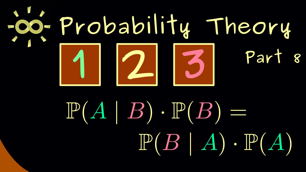
11 00:00:53,931 –> 00:01:03,992 Which leads us for left-hand side to P(A|B) times P(B) and on the right hand side it leads us to P(B|A) times P(A).

12 00:01:04,471 –> 00:01:08,144 and in fact, this is what we call Bayes’s theorem.

13 00:01:08,571 –> 00:01:16,001 In this order it’s easy to remember, because here we have the condition B and P(B) and here the condition A and P(A).

14 00:01:16,429 –> 00:01:20,743 Ok, at the end of the video I can show you how we can use this formula.

15 00:01:20,943 –> 00:01:25,141 However before we do this lets talk about the law of total probability.

16 00:01:25,529 –> 00:01:29,446 It tells us which possibilities we have to split up a probability.

17 00:01:29,814 –> 00:01:37,196 So as always we choose a probability space given by a sample space Omega, a sigma algebra A and the probability measure P.

18 00:01:37,557 –> 00:01:41,254 and now we want to calculate the probability of a subset A.

19 00:01:41,454 –> 00:01:44,543 So the question is: how can we split up P(A)?

20 00:01:45,271 –> 00:01:48,528 Now, one possibility would be to choose another set B.

21 00:01:48,929 –> 00:01:52,376 In the picture we can also visualize this maybe like this.

22 00:01:52,576 –> 00:01:57,578 So the set B is here and you immediately see how this set A is divided now.

23 00:01:57,886 –> 00:02:01,813 We get this, because we have the set B and the complement of B.

24 00:02:02,457 –> 00:02:07,170 and of course both together in a union gives us the whole sample space Omega.

25 00:02:07,370 –> 00:02:10,866 Important to note here is, this is indeed a disjoint union.

26 00:02:11,543 –> 00:02:15,459 Therefore this division here works no matter which event A we choose.

27 00:02:15,659 –> 00:02:18,569 and this is now what we can put into a formula.

28 00:02:18,769 –> 00:02:23,058 So we have P(A), where we can write A as a disjoint union.

29 00:02:23,500 –> 00:02:29,123 Namely the union of the upper part here we have in B, with the other part we have in B^c.

30 00:02:29,514 –> 00:02:35,367 and because this is a disjoint union, we can use the property of the measure and write it as a sum.

31 00:02:35,743 –> 00:02:40,438 So we have the probability of this intersection + the probability of that intersection.

32 00:02:40,638 –> 00:02:44,957 Now as before an intersection we can rewrite as a conditional probability.

33 00:02:45,557 –> 00:02:49,536 For the first one we write P(A|B) times P(B).

34 00:02:49,736 –> 00:02:54,087 and for the second one we use the same formula, but now with the complement of B.

35 00:02:54,287 –> 00:03:01,410 So you see, this is a nice formula, we can use to calculate the probability of A, when we know these 4 probabilities here.

36 00:03:01,800 –> 00:03:05,717 However the law of total probability goes even further.

37 00:03:05,917 –> 00:03:11,573 We can also deal with the case that we don’t have only one set B, but countably many.

38 00:03:11,957 –> 00:03:15,888 So we could have 2, 3 or even infinitely many.

39 00:03:16,088 –> 00:03:21,553 Hence we simply say we have B_i, where i comes from the index set that is a subset of the natural numbers.

40 00:03:21,943 –> 00:03:25,420 and of course we have to generalize this property here.

41 00:03:25,771 –> 00:03:29,788 This means that the union of all these sets is equal to Omega.

42 00:03:29,988 –> 00:03:33,829 and in addition as before, it needs to be a disjoint union.

43 00:03:34,029 –> 00:03:37,293 Now lets also visualize this in a picture.

44 00:03:37,614 –> 00:03:43,243 There is our sample space Omega again and now we don’t just find one set B, but a lot of them.

45 00:03:43,714 –> 00:03:46,957 For example such a decomposition of Omega could look like this.

46 00:03:47,600 –> 00:03:51,884 and here please don’t forget it’s possible that we have infinitely many sets B_i.

47 00:03:52,084 –> 00:03:57,015 Therefore in this picture they would get thinner and thinner when we go in this direction, for example.

48 00:03:57,215 –> 00:04:00,070 Of course there are a lot possibilities to visualize this.

49 00:04:00,270 –> 00:04:06,138 However the important part here is that we also have a set A of which we want to calculate the probability.

50 00:04:06,600 –> 00:04:10,057 In fact this now works exactly with the same steps as before.

51 00:04:10,686 –> 00:04:14,559 So first we can write a set A as a disjoint union.

52 00:04:14,759 –> 00:04:21,532 Of course this is again, the intersection with the B_i’s. Which means in the picture we just put all these parts here together.

53 00:04:21,732 –> 00:04:27,395 Ok then because it’s a disjoint union, we can use the sigma additivity of the measure.

54 00:04:27,829 –> 00:04:32,502 So we get out this sum for the probabilities or a series when we have infinitely many.

55 00:04:32,702 –> 00:04:36,343 However in both cases we can us the conditional probabilities again.

56 00:04:36,771 –> 00:04:42,029 So we have the sum of P(A|B_i) times the probability of B_i.

57 00:04:42,229 –> 00:04:46,685 Now, this formula here is indeed the general law of total probability.

58 00:04:46,885 –> 00:04:50,608 And how we can apply we will see in the next example.

59 00:04:51,443 –> 00:04:55,639 Actually this is one of the most famous examples of probability theory.

60 00:04:56,043 –> 00:04:58,698 It’s the so called Monty Hall problem.

61 00:04:58,898 –> 00:05:03,922 and because it is so well known, i don’t want to go into the whole history and the details.

62 00:05:04,122 –> 00:05:08,029 We just use it to compute a probability with the 2 laws above.

63 00:05:08,351 –> 00:05:11,635 However I still have to explain how this whole puzzle works.

64 00:05:11,835 –> 00:05:18,436 So we have a game show with 3 doors, where there is one door with a car behind and 2 doors with a goat behind.

65 00:05:18,729 –> 00:05:22,744 and now lets assume that the car would be the better price to win.

66 00:05:23,043 –> 00:05:25,543 Ok then the game works in 3 steps.

67 00:05:26,057 –> 00:05:29,350 First you pick a door. Lets say you pick door 1.

68 00:05:29,550 –> 00:05:33,870 Afterwards in the second step the showmaster always shows you a goat.

69 00:05:34,070 –> 00:05:36,638 So he opens one of the 2 remaining doors.

70 00:05:36,838 –> 00:05:39,771 and maybe lets say here he opens door 3.

71 00:05:40,257 –> 00:05:43,760 and then in the last step you have to do your final pick.

72 00:05:44,043 –> 00:05:47,292 So you can either keep the original door or you can switch.

73 00:05:47,492 –> 00:05:52,373 and now I can already tell you, switching has the higher probability to getting the car.

74 00:05:52,986 –> 00:05:56,688 Therefore if you want the goat you should stay at the original door.

75 00:05:57,000 –> 00:06:00,546 However no matter what you want, we can calculate the probabilities now.

76 00:06:00,986 –> 00:06:04,489 Here please note, the names for the doors are arbitrary.

77 00:06:04,654 –> 00:06:09,542 So we can call the first door we pick just (1).

78 00:06:10,000 –> 00:06:13,486 Moreover we need some names for the events we consider here.

79 00:06:13,670 –> 00:06:17,498 Here c_j should be the event that the car is behind door j.

80 00:06:17,769 –> 00:06:23,450 In addition s_j should be event that in the second step the showmaster opens door j.

81 00:06:23,589 –> 00:06:26,823 Hence we already know some conditional probabilities.

82 00:06:27,099 –> 00:06:30,000 And in order to make our life a little bitte easier,

83 00:06:30,000 –> 00:06:39,069 Let’s only consider the case that the show master opens door 3. The other interesting case with S_2 can be described in the same way.

84 00:06:39,069 –> 00:06:43,967 Okay, so in this case we already some conditional probabilities.

85 00:06:44,864 –> 00:06:50,793 Namely the probability of s_3 under the condition c_3 has to be 0.

86 00:06:51,847 –> 00:06:53,752 The showmaster will never show you the car in the second step.

87 00:06:54,622 –> 00:06:57,450 He always opens a door with a goat.

88 00:06:57,488 –> 00:07:02,222 Therefore we also now the probability of s_3 under the condition c_2.

89 00:07:02,773 –> 00:07:06,511 Because this is what I told you, he opens one of the 2 remaining doors.

90 00:07:06,727 –> 00:07:08,547 Never the door you picked.

91 00:07:08,747 –> 00:07:11,532 So in this scenario here, he does not have a choice.

92 00:07:11,970 –> 00:07:15,247 Hence the conditional probability here is 1.

93 00:07:15,447 –> 00:07:20,973 Then the last remaining case would be where he has a choice. Therefore we say the probability is 1/2.

94 00:07:20,993 –> 00:07:25,707 So you see, just by knowing the problem we already get a lot of information.

95 00:07:26,346 –> 00:07:32,391 And please also note, here we didn’t define a sample space, sigma algebra or even a probability measure yet.

96 00:07:32,736 –> 00:07:39,834 Simply because we don’t need it. We just want to know what happens in any probability space, when we have these conditional probabilities.

97 00:07:40,121 –> 00:07:42,996 Indeed this will be our last step here.

98 00:07:43,643 –> 00:07:49,262 So we want to know: what is the probability of getting the car when I switch the door in the third step.

99 00:07:49,877 –> 00:07:52,422 And this is exactly given by this conditional probability.

100 00:07:52,710 –> 00:07:56,854 Now, maybe not so surprising now we can apply Bayes’s theorem here.

101 00:07:58,462 –> 00:07:59,840 Please recall what it tells us.

102 00:08:00,000 –> 00:08:05,899 We can exchange the order in the conditional probability here, when multiply with the probability of the last part.

103 00:08:06,025 –> 00:08:11,462 However we don’t have it on the left hand side. Therefore we have to divide here by the probability of s_3.

104 00:08:12,025 –> 00:08:15,460 Therefore often you see Bayes’s theorem in this formulation.

105 00:08:16,426 –> 00:08:21,712 Ok, now here on the right-hand side we have a problem, because we don’t know what P(s_3) is.

106 00:08:21,712 –> 00:08:28,132 However we have all the conditional probabilities here. Therefore we can use the law of total probability.

107 00:08:28,813 –> 00:08:32,324 Hence in the denominator we get a sum with 3 parts.

108 00:08:32,482 –> 00:08:38,701 Namely we sum over P(s_3|c_j) times the probability of c_j.

109 00:08:39,244 –> 00:08:42,359 and there we can put in our conditional probabilities.

110 00:08:42,722 –> 00:08:47,571 Ok then lets start in the numerator. This probability here is 1.

111 00:08:47,946 –> 00:08:51,036 and the same we find here in the denominator as well.

112 00:08:51,513 –> 00:08:55,894 Then on the right hand side we find a conditional probability that is 0.

113 00:08:56,445 –> 00:08:59,778 and then the last remaining one on the left is 1/2.

114 00:09:00,000 –> 00:09:05,727 Ok now you see the last ingredient we need would be the probability of c_2 and c_1.

115 00:09:06,134 –> 00:09:10,346 and there of course we have the assumption that it’s the same probability.

116 00:09:10,458 –> 00:09:15,425 So we assume fair game. Each door has the same probability for getting the price.

117 00:09:15,976 –> 00:09:20,083 and by having 3 doors this would mean we have the probability 1/3.

118 00:09:20,808 –> 00:09:25,869 Ok, now we have substituted everything with numbers, such that we can simply compute.

119 00:09:25,869 –> 00:09:27,643 and we get out 2/3.

120 00:09:28,170 –> 00:09:32,819 So indeed we get out the result that in this scenario switching is beneficial.

121 00:09:34,579 –> 00:09:42,339 However of course the goal here was not winning a car, but rather seeing the application of Bayes’s theorem and law of total probability.

122 00:09:42,339 –> 00:09:48,837 Ok with this I think it’s good enough for today and I hope I see you in the next video. Have a nice day and Bye! :) :)

Q1: Let $(\Omega, \mathcal{A}, \mathbb{P})$ be a probability space and $A,B \in \mathcal{A}$. What is the correct formulation for Bayes’s theorem?

A1: $$ \mathbb{P}(A \mid B) \cdot \mathbb{P}(B) = \mathbb{P}(A \mid B)\cdot \mathbb{P}(B) $$

A2: $$ \mathbb{P}(A \mid B) \cdot \mathbb{P}(B) = \mathbb{P}(B \mid B)\cdot \mathbb{P}(B) $$

A3: $$ \mathbb{P}(A \mid B) \cdot \mathbb{P}(B) = \mathbb{P}(B \mid A)\cdot \mathbb{P}(A) $$

A4: $$ \mathbb{P}(A \mid B) \cdot \mathbb{P}(B) = \mathbb{P}(A \mid B)\cdot \mathbb{P}(A) $$

Q2: Let $(\Omega, \mathcal{A}, \mathbb{P})$ be a probability space, $B_1, B_2, B_3 \in \mathcal{A}$ pairwise disjoint with $B_1 \cup B_2 \cup B_3 = \Omega$. What is the correct formulation for the law of total probability?

A1: $$\mathbb{P}(A) = \mathbb{P}(A \mid B_1) \cdot \mathbb{P}(B_1) +\mathbb{P}(A \mid B_2) \cdot \mathbb{P}(B_2) + \mathbb{P}(A \mid B_3) \cdot \mathbb{P}(B_3) $$

A2: $$\mathbb{P}(A) = \mathbb{P}(A \mid B_1) +\mathbb{P}(A \mid B_2) + \mathbb{P}(A \mid B_3) $$

A3: $$\mathbb{P}(A) = \mathbb{P}(B_1) +\mathbb{P}(B_2) + \mathbb{P}(B_3) $$

A4: $$\mathbb{P}(A) = \mathbb{P}(B_1 \mid A) \cdot \mathbb{P}(B_1) +\mathbb{P}(B_2 \mid A) \cdot \mathbb{P}(B_2) + \mathbb{P}(B_3 \mid A) \cdot \mathbb{P}(B_3) $$

Q3: Consider the Monty Hall problem. What is the probability of getting the car if you don’t switch doors in the last step?

A1: $1$

A2: $\frac{1}{2}$

A3: $\frac{1}{3}$

A4: $\frac{2}{3}$

A5: $0$