-
Title: Local Extreme and Rolle’s Theorem
-
Series: Real Analysis
-
Chapter: Differentiable Functions
-
YouTube-Title: Real Analysis 40 | Local Extreme and Rolle’s Theorem
-
Bright video: Watch on YouTube
-
Dark video: Watch on YouTube
-
Ad-free video: Watch Vimeo video
-
Original video for YT-Members (bright): Watch on YouTube
-
Original video for YT-Members (dark): Watch on YouTube
-
Forum: Ask a question in Mattermost
-
Quiz: Test your knowledge
-
Dark-PDF: Download PDF version of the dark video
-
Print-PDF: Download printable PDF version
-
Exercise Download PDF sheets
-
Thumbnail (bright): Download PNG
-
Thumbnail (dark): Download PNG
-
Subtitle on GitHub: ra40_sub_eng.srt
-
Download bright video: Link on Vimeo
-
Download dark video: Link on Vimeo
-
Timestamps (n/a)
-
Subtitle in English
1 00:00:00,409 –> 00:00:02,349 Hello and welcome back to
2 00:00:02,359 –> 00:00:03,960 real analysis.
3 00:00:04,400 –> 00:00:05,849 And obviously, as always
4 00:00:05,860 –> 00:00:07,079 first, I want to thank all
5 00:00:07,090 –> 00:00:08,279 the nice people that support
6 00:00:08,289 –> 00:00:09,399 this channel on study or
7 00:00:09,409 –> 00:00:10,069 paypal.
8 00:00:10,489 –> 00:00:11,680 Now we’ve almost reached
9 00:00:11,689 –> 00:00:12,960 a point in the series where
10 00:00:12,970 –> 00:00:14,399 we can talk about the famous
11 00:00:14,409 –> 00:00:16,229 mean value theorem.
12 00:00:16,510 –> 00:00:17,909 However, before we are able
13 00:00:17,920 –> 00:00:19,209 to prove it, we first have
14 00:00:19,219 –> 00:00:20,760 to talk about local extrema
15 00:00:20,979 –> 00:00:22,629 and the theorem of Rolle.
16 00:00:23,280 –> 00:00:24,500 Hence today, we will do the
17 00:00:24,510 –> 00:00:25,659 whole ground work we will
18 00:00:25,670 –> 00:00:27,459 need for the mean value theorem.
19 00:00:27,809 –> 00:00:29,030 So let’s immediately start
20 00:00:29,040 –> 00:00:30,250 with the definition of a
21 00:00:30,260 –> 00:00:32,180 local maximum for
22 00:00:32,189 –> 00:00:32,418 this.
23 00:00:32,430 –> 00:00:34,369 Let’s fix an interval I and
24 00:00:34,380 –> 00:00:35,549 a function F.
25 00:00:35,930 –> 00:00:37,229 Now, in order to understand
26 00:00:37,240 –> 00:00:38,919 what we want to define let’s
27 00:00:38,930 –> 00:00:40,389 visualize the graph.
28 00:00:40,750 –> 00:00:42,259 So maybe we have something
29 00:00:42,270 –> 00:00:44,150 like this and the
30 00:00:44,159 –> 00:00:45,610 point like this, we want
31 00:00:45,619 –> 00:00:47,360 to call a local maximum
32 00:00:47,930 –> 00:00:49,200 or more concretely, we are
33 00:00:49,209 –> 00:00:50,700 interested in the point X
34 00:00:50,709 –> 00:00:52,439 zero at the X axis.
35 00:00:52,659 –> 00:00:54,340 In this case, you would say
36 00:00:54,349 –> 00:00:55,900 the function F has a local
37 00:00:55,909 –> 00:00:57,380 maximum at this point.
38 00:00:57,909 –> 00:00:58,290 OK.
39 00:00:58,299 –> 00:00:59,500 And now of course, we should
40 00:00:59,509 –> 00:01:00,979 think about what this should
41 00:01:00,990 –> 00:01:02,180 essentially mean.
42 00:01:02,549 –> 00:01:03,970 Now, the value of the function
43 00:01:03,979 –> 00:01:05,540 at this point does not have
44 00:01:05,550 –> 00:01:06,900 to be the maximum of the
45 00:01:06,910 –> 00:01:07,500 function.
46 00:01:07,980 –> 00:01:09,360 However, it should be
47 00:01:09,370 –> 00:01:11,230 maximal when we only consider
48 00:01:11,239 –> 00:01:12,529 a neighborhood around this
49 00:01:12,540 –> 00:01:13,000 point.
50 00:01:13,330 –> 00:01:14,949 Or to be more precise, we
51 00:01:14,959 –> 00:01:16,470 only consider a neighborhood
52 00:01:16,480 –> 00:01:18,220 around the point X zero on
53 00:01:18,230 –> 00:01:19,129 the X axis.
54 00:01:19,760 –> 00:01:21,639 And this one we simply call
55 00:01:21,650 –> 00:01:22,139 you.
56 00:01:22,629 –> 00:01:24,040 So we just need a neighborhood
57 00:01:24,050 –> 00:01:25,080 in the real numbers.
58 00:01:25,089 –> 00:01:26,129 And if you want, you can
59 00:01:26,139 –> 00:01:27,720 choose an epsilon neighborhood.
60 00:01:28,230 –> 00:01:29,459 And of course, it just have
61 00:01:29,470 –> 00:01:31,139 to be small enough such that
62 00:01:31,150 –> 00:01:32,720 our condition here holds.
63 00:01:33,190 –> 00:01:34,610 Hence, in the formula, this
64 00:01:34,620 –> 00:01:36,180 would mean that F of X
65 00:01:36,190 –> 00:01:37,980 zero is equal to the
66 00:01:37,989 –> 00:01:39,690 maximum of the function when
67 00:01:39,699 –> 00:01:41,489 we only consider points from
68 00:01:41,500 –> 00:01:42,300 the neighborhood.
69 00:01:42,769 –> 00:01:44,690 Hence, we have X in U
70 00:01:44,699 –> 00:01:46,139 intersected with I
71 00:01:46,790 –> 00:01:48,169 with this intersection, we
72 00:01:48,180 –> 00:01:49,540 also include points that
73 00:01:49,550 –> 00:01:50,900 lie on the boundary of the
74 00:01:50,910 –> 00:01:51,480 interval.
75 00:01:51,910 –> 00:01:53,309 Otherwise it’s exactly the
76 00:01:53,319 –> 00:01:54,949 same thing we explained here
77 00:01:54,959 –> 00:01:55,720 in the graph.
78 00:01:56,440 –> 00:01:57,900 And there, you also see we
79 00:01:57,910 –> 00:01:59,410 can do the same thing for
80 00:01:59,419 –> 00:02:00,580 a local minimum.
81 00:02:01,099 –> 00:02:02,620 Therefore, I would say let’s
82 00:02:02,629 –> 00:02:04,459 add this to our definition.
83 00:02:04,989 –> 00:02:06,650 So we say the function F
84 00:02:06,660 –> 00:02:08,220 has a local minimum at the
85 00:02:08,229 –> 00:02:09,429 point X zero.
86 00:02:10,110 –> 00:02:11,300 If there is a neighborhood
87 00:02:11,309 –> 00:02:12,889 of X zero also called
88 00:02:12,899 –> 00:02:14,619 U such that F of X
89 00:02:14,630 –> 00:02:16,059 zero is the minimum of the
90 00:02:16,070 –> 00:02:17,580 function when we restrict
91 00:02:17,589 –> 00:02:18,960 it to the neighborhood U.
92 00:02:19,490 –> 00:02:21,050 So you see it’s exactly the
93 00:02:21,059 –> 00:02:22,580 same definition as before,
94 00:02:22,669 –> 00:02:23,899 just with a minimum.
95 00:02:24,339 –> 00:02:25,559 Then finally, we have the
96 00:02:25,570 –> 00:02:27,080 last part of the definition
97 00:02:27,089 –> 00:02:28,470 which is about local
98 00:02:28,479 –> 00:02:29,119 extrema.
99 00:02:29,949 –> 00:02:31,559 In fact, this is just a name
100 00:02:31,570 –> 00:02:33,520 to combine both maximum and
101 00:02:33,529 –> 00:02:34,699 minimum from before.
102 00:02:35,179 –> 00:02:36,869 Hence we say F has a local
103 00:02:36,880 –> 00:02:38,779 extrem at X zero, if
104 00:02:38,789 –> 00:02:40,509 F has a local maximum or
105 00:02:40,520 –> 00:02:42,240 a local minimum at X zero.
106 00:02:42,639 –> 00:02:44,449 So you see this is not complicated
107 00:02:44,460 –> 00:02:46,229 at all, but maybe I still
108 00:02:46,240 –> 00:02:47,639 show you some sketches.
109 00:02:48,410 –> 00:02:49,979 Therefore, here in the coordinate
110 00:02:49,990 –> 00:02:51,600 system, we have our interval
111 00:02:51,610 –> 00:02:53,220 I as a bounded one.
112 00:02:53,720 –> 00:02:55,190 Then for example, the graph
113 00:02:55,199 –> 00:02:56,860 of F could look like this.
114 00:02:57,410 –> 00:02:58,500 And they, you see on the
115 00:02:58,509 –> 00:03:00,339 left boundary we have a local
116 00:03:00,350 –> 00:03:01,059 maximum.
117 00:03:01,610 –> 00:03:03,059 And on the right hand boundary,
118 00:03:03,070 –> 00:03:04,539 we have a local minimum.
119 00:03:04,750 –> 00:03:06,339 Moreover, another local
120 00:03:06,350 –> 00:03:08,059 maximum, we also find here
121 00:03:08,580 –> 00:03:10,360 also another local minimum
122 00:03:10,369 –> 00:03:11,500 we find here.
123 00:03:12,149 –> 00:03:13,240 So please don’t forget a
124 00:03:13,250 –> 00:03:14,529 local maximum could look
125 00:03:14,539 –> 00:03:15,149 like this.
126 00:03:15,830 –> 00:03:16,929 But of course, when we deal
127 00:03:16,940 –> 00:03:18,330 with differentiable functions,
128 00:03:18,339 –> 00:03:19,770 something like this cannot
129 00:03:19,779 –> 00:03:20,169 happen.
130 00:03:21,000 –> 00:03:22,279 In fact, for differential
131 00:03:22,289 –> 00:03:23,410 functions, we have a very
132 00:03:23,419 –> 00:03:24,889 nice necessary condition
133 00:03:24,899 –> 00:03:25,979 for local extrema.
134 00:03:26,429 –> 00:03:28,119 So let’s put this into a
135 00:03:28,130 –> 00:03:28,889 proposition.
136 00:03:29,479 –> 00:03:30,809 However, we don’t have this
137 00:03:30,820 –> 00:03:32,630 condition for boundary points.
138 00:03:32,639 –> 00:03:33,660 Therefore, I immediately
139 00:03:33,669 –> 00:03:35,309 choose an open interval as
140 00:03:35,320 –> 00:03:36,169 the domain.
141 00:03:36,380 –> 00:03:37,880 Now our assumption here is
142 00:03:37,889 –> 00:03:39,210 that at the point X zero,
143 00:03:39,220 –> 00:03:40,600 we are interested in the
144 00:03:40,610 –> 00:03:42,210 function is differentiable.
145 00:03:42,679 –> 00:03:44,339 And then we have the following
146 00:03:44,350 –> 00:03:46,199 implication if
147 00:03:46,210 –> 00:03:47,660 F has a local extremum at
148 00:03:47,669 –> 00:03:49,649 x zero, so a local maximum
149 00:03:49,660 –> 00:03:51,500 or minimum, then
150 00:03:51,509 –> 00:03:53,440 F prime of X zero
151 00:03:53,449 –> 00:03:54,899 is equal to zero.
152 00:03:55,520 –> 00:03:57,050 So the derivative has to
153 00:03:57,059 –> 00:03:58,380 vanish at this point.
154 00:03:59,100 –> 00:04:00,279 Now please immediately note
155 00:04:00,289 –> 00:04:01,940 here, this does not work
156 00:04:01,949 –> 00:04:03,000 the other way around.
157 00:04:03,410 –> 00:04:05,029 Now, both things we can immediately
158 00:04:05,039 –> 00:04:06,509 explain in a picture.
159 00:04:06,880 –> 00:04:08,270 For example, if we have a
160 00:04:08,279 –> 00:04:09,940 local maximum here, the
161 00:04:09,949 –> 00:04:11,559 slope at the point if it
162 00:04:11,570 –> 00:04:13,479 exists needs to be zero.
163 00:04:14,070 –> 00:04:15,369 So we have a tangent that
164 00:04:15,380 –> 00:04:16,350 is horizontal.
165 00:04:16,738 –> 00:04:18,170 However, this horizontal
166 00:04:18,178 –> 00:04:19,858 tangent can’t be sufficient
167 00:04:19,869 –> 00:04:21,010 for a local extremum
168 00:04:21,589 –> 00:04:23,220 because we also have it at
169 00:04:23,230 –> 00:04:25,140 this point for such a curve.
170 00:04:25,679 –> 00:04:27,059 And there at this point,
171 00:04:27,070 –> 00:04:28,640 we don’t have a local minimum
172 00:04:28,649 –> 00:04:30,040 and also not a local
173 00:04:30,049 –> 00:04:30,760 maximum.
174 00:04:31,369 –> 00:04:32,579 Therefore, please always
175 00:04:32,589 –> 00:04:34,010 have this direction here
176 00:04:34,019 –> 00:04:34,540 in mind.
177 00:04:35,239 –> 00:04:35,579 OK.
178 00:04:35,589 –> 00:04:37,000 Then I guess we are ready
179 00:04:37,010 –> 00:04:38,859 for the proof of this statement.
180 00:04:39,230 –> 00:04:40,950 And there we will distinguish
181 00:04:40,959 –> 00:04:41,850 two cases,
182 00:04:42,399 –> 00:04:44,019 namely, we first consider
183 00:04:44,029 –> 00:04:45,950 that F has a local maximum
184 00:04:45,959 –> 00:04:46,859 at X zero.
185 00:04:47,089 –> 00:04:48,859 And then obviously the second
186 00:04:48,869 –> 00:04:50,309 case will be that F has a
187 00:04:50,320 –> 00:04:52,049 local minimum at X zero.
188 00:04:52,540 –> 00:04:52,859 OK.
189 00:04:52,869 –> 00:04:54,170 Then by the definition of
190 00:04:54,179 –> 00:04:55,579 a local maximum, we can
191 00:04:55,589 –> 00:04:57,519 conclude that there is a
192 00:04:57,529 –> 00:04:58,940 neighborhood of X zero.
193 00:04:58,950 –> 00:05:00,100 We call you
194 00:05:00,750 –> 00:05:01,170 here.
195 00:05:01,179 –> 00:05:02,390 Very importantly, to note
196 00:05:02,399 –> 00:05:03,630 is because we have an inner
197 00:05:03,640 –> 00:05:04,959 point, we can choose the
198 00:05:04,970 –> 00:05:06,940 neighborhood inside the interval.
199 00:05:06,950 –> 00:05:08,869 AB otherwise we have the
200 00:05:08,880 –> 00:05:10,649 same property here, namely
201 00:05:10,660 –> 00:05:12,450 F of X zero is the maximum
202 00:05:12,459 –> 00:05:14,000 of the function when we only
203 00:05:14,010 –> 00:05:15,190 consider points from the
204 00:05:15,200 –> 00:05:15,890 neighborhood.
205 00:05:16,269 –> 00:05:17,480 Now, in the next step, what
206 00:05:17,489 –> 00:05:18,779 we can put in is that the
207 00:05:18,790 –> 00:05:20,579 function F is differentiable
208 00:05:20,589 –> 00:05:21,989 at our point X zero.
209 00:05:22,000 –> 00:05:23,730 This means we have a
210 00:05:23,739 –> 00:05:25,049 linearization around this
211 00:05:25,059 –> 00:05:26,709 point in general.
212 00:05:26,720 –> 00:05:28,279 This means we can write F
213 00:05:28,290 –> 00:05:30,190 of X as F of
214 00:05:30,209 –> 00:05:31,989 X zero plus X minus X
215 00:05:32,000 –> 00:05:33,910 zero times our slope function
216 00:05:33,920 –> 00:05:34,459 delta.
217 00:05:34,910 –> 00:05:36,239 And here please recall the
218 00:05:36,250 –> 00:05:38,059 important property for differentiability
219 00:05:38,070 –> 00:05:39,859 is that this function
220 00:05:39,869 –> 00:05:41,540 here is continuous at the
221 00:05:41,549 –> 00:05:42,540 point X zero.
222 00:05:42,980 –> 00:05:44,459 This is not what we can use
223 00:05:44,470 –> 00:05:45,839 to show that the slope at
224 00:05:45,850 –> 00:05:47,579 X zero is zero.
225 00:05:47,970 –> 00:05:48,859 Intuitively.
226 00:05:48,869 –> 00:05:50,220 It makes sense that we have
227 00:05:50,230 –> 00:05:51,739 it because if we would have
228 00:05:51,750 –> 00:05:53,130 a tangent with a positive
229 00:05:53,140 –> 00:05:55,059 slope, then we cannot have
230 00:05:55,070 –> 00:05:56,890 a local maximum here because
231 00:05:56,899 –> 00:05:58,470 the value will increase when
232 00:05:58,480 –> 00:05:59,510 we go to the right.
233 00:06:00,179 –> 00:06:01,779 Therefore, let’s try to
234 00:06:01,790 –> 00:06:02,769 prove this.
235 00:06:03,140 –> 00:06:04,709 So we assume that at the
236 00:06:04,720 –> 00:06:06,359 point X zero, the function
237 00:06:06,369 –> 00:06:07,570 delta which is the
238 00:06:07,579 –> 00:06:09,309 derivative is greater than
239 00:06:09,320 –> 00:06:09,929 zero.
240 00:06:10,380 –> 00:06:12,269 Now, since we have continuity,
241 00:06:12,279 –> 00:06:14,089 we also know the function
242 00:06:14,100 –> 00:06:15,359 is greater than zero in a
243 00:06:15,369 –> 00:06:16,700 small neighborhood around
244 00:06:16,709 –> 00:06:18,410 X zero, let’s call the
245 00:06:18,420 –> 00:06:19,489 neighborhood V.
246 00:06:19,500 –> 00:06:20,720 And of course, we can choose
247 00:06:20,730 –> 00:06:22,149 it as a subset of U.
248 00:06:22,709 –> 00:06:23,910 Now, this is the important
249 00:06:23,920 –> 00:06:25,809 property we can use to construct
250 00:06:25,820 –> 00:06:27,429 the contradiction as a
251 00:06:27,440 –> 00:06:28,010 reminder.
252 00:06:28,019 –> 00:06:29,329 Another way to interpret
253 00:06:29,339 –> 00:06:31,010 this property here is to think
254 00:06:31,019 –> 00:06:31,929 of secants.
255 00:06:32,329 –> 00:06:33,600 If the slope of the tangent
256 00:06:33,609 –> 00:06:34,959 is positive, then you also
257 00:06:34,970 –> 00:06:36,040 find a small neighborhood
258 00:06:36,049 –> 00:06:37,579 around X zero such that the
259 00:06:37,589 –> 00:06:39,179 slopes of the secants is
260 00:06:39,190 –> 00:06:40,350 positive as well.
261 00:06:40,850 –> 00:06:42,690 However, now if we have this,
262 00:06:42,700 –> 00:06:44,399 we cannot have a maximum
263 00:06:44,410 –> 00:06:46,190 at X zero, you immediately
264 00:06:46,200 –> 00:06:47,910 see this in the picture because
265 00:06:47,920 –> 00:06:49,079 on the right hand side of
266 00:06:49,089 –> 00:06:50,809 X zero, we find larger
267 00:06:50,820 –> 00:06:52,399 values than at the point
268 00:06:52,410 –> 00:06:52,989 X zero.
269 00:06:53,649 –> 00:06:54,980 We can also show this when
270 00:06:54,989 –> 00:06:56,679 we use our identity here
271 00:06:57,309 –> 00:06:59,010 because here, if X is in
272 00:06:59,019 –> 00:07:00,170 the neighborhood V we
273 00:07:00,179 –> 00:07:01,399 have a positive number.
274 00:07:01,820 –> 00:07:03,290 And if we choose X on the
275 00:07:03,299 –> 00:07:04,730 right hand side of X zero,
276 00:07:04,739 –> 00:07:06,679 this is also positive number.
277 00:07:07,049 –> 00:07:08,730 In summary, all points X
278 00:07:08,739 –> 00:07:10,010 in the neighborhood fulfill
279 00:07:10,019 –> 00:07:11,790 that F of X is greater
280 00:07:11,799 –> 00:07:13,769 than F of X zero, which
281 00:07:13,779 –> 00:07:15,410 simply means that F of X
282 00:07:15,420 –> 00:07:16,950 zero is not a local
283 00:07:16,959 –> 00:07:17,690 maximum.
284 00:07:18,209 –> 00:07:18,440 OK.
285 00:07:18,450 –> 00:07:19,720 Then let’s look at the second
286 00:07:19,730 –> 00:07:21,630 possibility here that F prime
287 00:07:21,640 –> 00:07:23,320 of X zero is less than
288 00:07:23,329 –> 00:07:23,880 zero.
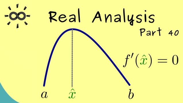
289 00:07:24,279 –> 00:07:25,480 There, you see we can just
290 00:07:25,489 –> 00:07:27,000 flip the picture from before
291 00:07:27,019 –> 00:07:28,579 and do the same argumentation
292 00:07:28,589 –> 00:07:29,019 again.
293 00:07:29,440 –> 00:07:30,779 So we can take a neighborhood
294 00:07:30,790 –> 00:07:32,720 V in you such that we have
295 00:07:32,730 –> 00:07:33,850 the negative slope in the
296 00:07:33,859 –> 00:07:34,820 whole neighborhood.
297 00:07:35,149 –> 00:07:36,130 Now, the only thing we have
298 00:07:36,140 –> 00:07:37,529 to change from before is
299 00:07:37,540 –> 00:07:38,980 that we now look at the left
300 00:07:38,989 –> 00:07:40,940 hand side because then
301 00:07:40,950 –> 00:07:42,619 both factors in the product
302 00:07:42,630 –> 00:07:44,010 on the right hand side are
303 00:07:44,019 –> 00:07:45,380 less than zero.
304 00:07:45,820 –> 00:07:47,290 Hence, the product itself
305 00:07:47,299 –> 00:07:48,459 is positive again,
306 00:07:49,140 –> 00:07:50,480 which gives us exactly the
307 00:07:50,489 –> 00:07:52,339 same contradiction as before.
308 00:07:52,790 –> 00:07:54,010 Therefore, in summary, we
309 00:07:54,019 –> 00:07:55,790 know these two cases here
310 00:07:55,799 –> 00:07:57,380 are not possible at all.
311 00:07:57,809 –> 00:07:59,239 So the only possibility that
312 00:07:59,250 –> 00:08:00,920 remains is that F prime is
313 00:08:00,929 –> 00:08:02,269 exactly zero,
314 00:08:02,690 –> 00:08:04,130 which is exactly what we
315 00:08:04,140 –> 00:08:05,119 wanted to prove.
316 00:08:05,390 –> 00:08:06,649 Now, to finish the proof,
317 00:08:06,660 –> 00:08:08,279 we just have to do this second
318 00:08:08,290 –> 00:08:10,269 case, which means now instead
319 00:08:10,279 –> 00:08:11,630 of a maximum, we consider
320 00:08:11,640 –> 00:08:13,200 that F has a local minimum
321 00:08:13,209 –> 00:08:13,910 at X zero.
322 00:08:14,220 –> 00:08:15,450 However, I don’t think I
323 00:08:15,459 –> 00:08:17,049 have to write this down because
324 00:08:17,059 –> 00:08:18,709 now we have all the ideas
325 00:08:18,720 –> 00:08:19,899 and you can do a similar
326 00:08:19,910 –> 00:08:21,089 proof as before.
327 00:08:21,670 –> 00:08:22,970 In fact, what I want to do
328 00:08:22,980 –> 00:08:24,019 in the next minutes is to
329 00:08:24,029 –> 00:08:25,690 show you the important theorem
330 00:08:25,700 –> 00:08:27,649 of Rolle this one is
331 00:08:27,660 –> 00:08:29,549 applicable if we have a differentiable
332 00:08:29,559 –> 00:08:31,470 function on a compact interval.
333 00:08:32,010 –> 00:08:33,150 Now it’s important that we
334 00:08:33,159 –> 00:08:34,808 have these two boundary points
335 00:08:34,820 –> 00:08:36,710 A and B because we
336 00:08:36,719 –> 00:08:37,799 need the assumption that
337 00:08:37,808 –> 00:08:39,599 F of A is equal to F of
338 00:08:39,609 –> 00:08:40,000 B.
339 00:08:40,599 –> 00:08:42,169 Now in a picture in a graph,
340 00:08:42,179 –> 00:08:43,450 this would mean we start
341 00:08:43,460 –> 00:08:45,169 here at a given value and
342 00:08:45,179 –> 00:08:46,200 then the function can do
343 00:08:46,210 –> 00:08:48,119 a lot of things, but we end
344 00:08:48,130 –> 00:08:49,510 at the same value again,
345 00:08:50,150 –> 00:08:51,609 then the claim will be that
346 00:08:51,619 –> 00:08:53,190 we find at least one point
347 00:08:53,200 –> 00:08:54,390 where we have a horizontal
348 00:08:54,400 –> 00:08:56,260 tangent and this point
349 00:08:56,270 –> 00:08:58,190 on the X axis we will call
350 00:08:58,200 –> 00:08:59,010 X hat.
351 00:08:59,510 –> 00:09:01,020 In other words, we find X
352 00:09:01,030 –> 00:09:02,710 hat in the interval such
353 00:09:02,719 –> 00:09:04,330 that F prime of X hat is
354 00:09:04,340 –> 00:09:06,210 equal to 01
355 00:09:06,219 –> 00:09:07,450 important part here is that
356 00:09:07,460 –> 00:09:09,210 X hat is not a boundary
357 00:09:09,219 –> 00:09:09,690 point.
358 00:09:09,700 –> 00:09:10,969 So we have an inner point
359 00:09:10,979 –> 00:09:11,950 of the interval.
360 00:09:12,549 –> 00:09:13,030 OK.
361 00:09:13,059 –> 00:09:14,659 I would say Rolle’s theorem
362 00:09:14,669 –> 00:09:16,289 here seems very natural.
363 00:09:16,780 –> 00:09:18,030 If we have such a function
364 00:09:18,039 –> 00:09:19,479 like this, there should be
365 00:09:19,489 –> 00:09:21,070 a local minimum or a local
366 00:09:21,080 –> 00:09:22,119 maximum somewhere.
367 00:09:22,900 –> 00:09:24,020 Therefore, let’s immediately
368 00:09:24,030 –> 00:09:25,309 try to prove it.
369 00:09:26,070 –> 00:09:27,190 Let’s again, start with a
370 00:09:27,200 –> 00:09:28,909 simple case namely that the
371 00:09:28,919 –> 00:09:30,700 function F is constant.
372 00:09:31,010 –> 00:09:32,960 Then of course, it’s differentiable
373 00:09:32,969 –> 00:09:34,169 and fulfills the condition
374 00:09:34,179 –> 00:09:35,909 that F of A is equal to F
375 00:09:35,919 –> 00:09:36,479 of B.
376 00:09:36,510 –> 00:09:38,400 But also the derivative is
377 00:09:38,409 –> 00:09:39,450 equal to zero.
378 00:09:39,890 –> 00:09:41,570 And this holds for all X
379 00:09:41,580 –> 00:09:42,729 in the whole interval.
380 00:09:43,159 –> 00:09:44,570 So we can simply choose any
381 00:09:44,580 –> 00:09:46,250 point for X hat and we are
382 00:09:46,260 –> 00:09:46,890 finished.
383 00:09:47,580 –> 00:09:48,900 Hence, the only interesting
384 00:09:48,909 –> 00:09:50,840 case is that F is not a
385 00:09:50,849 –> 00:09:51,909 constant function.
386 00:09:52,460 –> 00:09:52,849 OK.
387 00:09:52,859 –> 00:09:54,770 And now we can use that F
388 00:09:54,780 –> 00:09:56,650 is defined on a compact set.
389 00:09:56,729 –> 00:09:58,599 And by assumption differentiable
390 00:09:58,950 –> 00:10:00,510 which in particular means
391 00:10:00,520 –> 00:10:02,090 it’s a continuous function.
392 00:10:02,739 –> 00:10:04,679 And for these, we know the
393 00:10:04,690 –> 00:10:06,559 image of a compact set is
394 00:10:06,570 –> 00:10:08,080 also a compact set.
395 00:10:08,539 –> 00:10:09,820 This is what we have proven
396 00:10:09,830 –> 00:10:11,159 in part 30.
397 00:10:11,739 –> 00:10:13,020 In particular, we have proven
398 00:10:13,030 –> 00:10:14,320 that we always find the point
399 00:10:14,330 –> 00:10:15,849 X minus where the minimum
400 00:10:15,859 –> 00:10:17,650 occurs and the point X
401 00:10:17,659 –> 00:10:19,450 plus where the maximum occurs.
402 00:10:20,010 –> 00:10:21,440 Now, of course, one of the
403 00:10:21,450 –> 00:10:22,799 points could lie on the
404 00:10:22,809 –> 00:10:23,690 boundary.
405 00:10:23,969 –> 00:10:25,539 However, because the function
406 00:10:25,549 –> 00:10:27,419 is not constant, the other
407 00:10:27,429 –> 00:10:28,440 one cannot.
408 00:10:28,979 –> 00:10:30,440 And exactly this one, we
409 00:10:30,450 –> 00:10:32,000 can choose as x hat.
410 00:10:32,619 –> 00:10:33,979 Therefore, this means we
411 00:10:33,989 –> 00:10:35,250 have the maximum or the
412 00:10:35,260 –> 00:10:37,179 minimum in the middle somewhere.
413 00:10:37,609 –> 00:10:39,130 In fact, it’s the global
414 00:10:39,140 –> 00:10:40,510 maximum or minimum,
415 00:10:41,039 –> 00:10:42,950 which is of course also a
416 00:10:42,960 –> 00:10:43,909 local one.
417 00:10:44,340 –> 00:10:45,890 Hence, we can simply use
418 00:10:45,900 –> 00:10:47,429 the proposition from before
419 00:10:48,219 –> 00:10:49,869 which tells us that the derivative
420 00:10:49,880 –> 00:10:51,340 vanishes at the local
421 00:10:51,349 –> 00:10:52,109 extremum.
422 00:10:52,729 –> 00:10:54,190 And with this, the proof
423 00:10:54,200 –> 00:10:55,049 is finished.
424 00:10:55,840 –> 00:10:57,489 In fact, this nice theorem
425 00:10:57,500 –> 00:10:58,929 of Rolle we can use in the
426 00:10:58,940 –> 00:11:00,840 next video because
427 00:11:00,849 –> 00:11:02,500 there we will prove the famous
428 00:11:02,510 –> 00:11:04,250 mean value theorem.
429 00:11:04,619 –> 00:11:05,830 Therefore, I hope I see you
430 00:11:05,840 –> 00:11:07,289 there and have a nice day.
431 00:11:07,349 –> 00:11:08,130 Bye.
-
Quiz Content
Q1: Let $f \colon [a,b] \rightarrow \mathbb{R}$ be a function and $x_0 \in [a,b]$. What is the correct definition? $f$ has a local maximum at $x_0$ if
A1: there is $y \in \mathbb{R}$ with $y = \max{ f(x) $ $ \mid x \in [a,b] }.$
A2: there is a neighbourhood $U$ of $x_0$ in $\mathbb{R}$ such that $ f(x_0) = \max{ f(x) $ $ \mid x \in [a,b] }.$
A3: there is a neighbourhood $U$ of $x_0$ in $\mathbb{R}$ such that $f(x_0) = \max{ f(x) $ $ \mid x \in U \cap [a,b] }.$
A4: there is a neighbourhood $U$ of $x_0$ in $\mathbb{R}$ such that $f(x_0) = \max{ y $ $ \mid y \in U \cap [a,b] }.$
Q2: Let $f \colon [a,b] \rightarrow \mathbb{R}$ be a function and $x_0 \in [a,b]$. When do we say that $f$ has a local extremum at $x_0$?
A1: $f$ has a local maximum and a local minimum at $x_0$.
A2: $f$ has a local maximum or a local minimum at $x_0$.
A3: $f^\prime(x_0) = 0$.
Q3: Let $f \colon [a,b] \rightarrow \mathbb{R}$ be a differentiable function and $x_0 \in (a,b)$. Which implication is not correct?
A1: $f$ has a local maximum at $x_0$ $~\Rightarrow~$ $f^\prime(x_0) = 0$
A2: $f$ has a local minimum at $x_0$ $~\Rightarrow~$ $f^\prime(x_0) = 0$
A3: $f^\prime(x_0) = 0$ $~\Rightarrow~$ $f$ has a local extremum at $x_0$
A4: $f^\prime(x_0) \neq 0$ $~\Rightarrow~$ $f$ has not a local minimum at $x_0$
Q4: Let $f \colon [a,b] \rightarrow \mathbb{R}$ be a differentiable function with $f(a) = f(b)$. Which claim is correct?
A1: There is $\hat{x}$ with $f^\prime(\hat{x}) = 0$.
A2: There is $\hat{x}$ with $f(\hat{x}) = 0$.
A3: There is $\hat{x}$ with $f^\prime(\hat{x}) = f(\hat{x})$.
A4: There is $\hat{x}$ with $f^\prime(\hat{x}) = 1$.
-
Last update: 2025-09