1 00:00:00,389 –> 00:00:02,289 Hello and welcome back to

2 00:00:02,299 –> 00:00:03,859 real analysis.

3 00:00:04,289 –> 00:00:05,889 And first many, many thanks

4 00:00:05,900 –> 00:00:07,130 to all the nice people that

5 00:00:07,139 –> 00:00:08,500 support this channel on Steady

6 00:00:08,510 –> 00:00:09,220 or paypal.

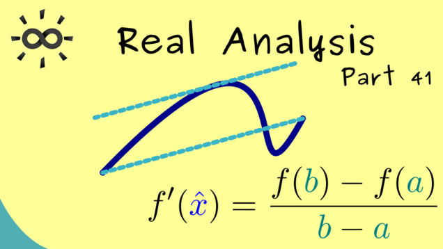
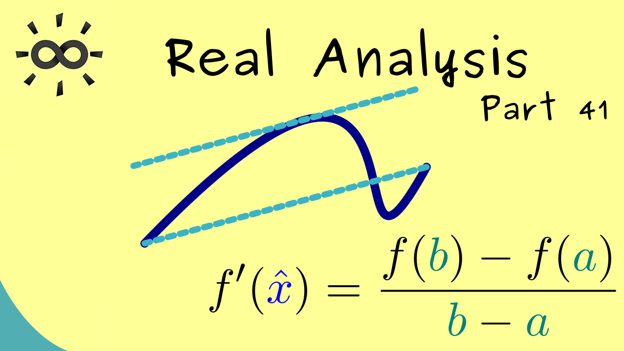
7 00:00:09,699 –> 00:00:11,449 Now today, in part 41 we

8 00:00:11,460 –> 00:00:12,680 will finally talk about the

9 00:00:12,689 –> 00:00:13,979 famous mean value

10 00:00:13,989 –> 00:00:14,770 theorem.

11 00:00:15,100 –> 00:00:16,850 Indeed, this theorem we can

12 00:00:16,860 –> 00:00:18,360 immediately visualize in

13 00:00:18,370 –> 00:00:19,180 a nice way.

14 00:00:19,700 –> 00:00:21,170 Now I can already tell you

15 00:00:21,180 –> 00:00:22,850 the mean value theorem applies

16 00:00:22,860 –> 00:00:24,059 to all functions that are

17 00:00:24,069 –> 00:00:25,920 defined on a compact interval

18 00:00:25,930 –> 00:00:27,120 and differentiable.

19 00:00:27,620 –> 00:00:28,629 Therefore, let’s call the

20 00:00:28,639 –> 00:00:29,909 interval on the X axis

21 00:00:29,920 –> 00:00:31,389 simply A B.

22 00:00:32,060 –> 00:00:32,459 OK.

23 00:00:32,470 –> 00:00:33,880 And now we look at the mean

24 00:00:33,889 –> 00:00:35,159 slope of the function

25 00:00:35,889 –> 00:00:37,470 which is the slope of this

26 00:00:37,479 –> 00:00:37,950 second.

27 00:00:38,639 –> 00:00:39,959 And of course, we can immediately

28 00:00:39,970 –> 00:00:41,819 calculate this by F of B

29 00:00:41,830 –> 00:00:43,819 minus F of A divided by

30 00:00:43,830 –> 00:00:45,069 B minus A.

31 00:00:45,590 –> 00:00:46,860 Now, the claim of the mean

32 00:00:46,869 –> 00:00:48,209 value theorem is that we

33 00:00:48,220 –> 00:00:49,939 also find a tangent with

34 00:00:49,950 –> 00:00:51,020 the same slope.

35 00:00:51,580 –> 00:00:52,740 So in the picture, this would

36 00:00:52,750 –> 00:00:54,159 mean we can push this

37 00:00:54,169 –> 00:00:56,130 sequence until we find the

38 00:00:56,139 –> 00:00:57,139 correct slope

39 00:00:58,060 –> 00:00:59,590 and the corresponding point

40 00:00:59,599 –> 00:01:01,459 in the interval A B we call

41 00:01:01,470 –> 00:01:03,450 X hat all in

42 00:01:03,459 –> 00:01:05,089 all this is already the

43 00:01:05,099 –> 00:01:07,010 whole mean value theorem.

44 00:01:07,480 –> 00:01:09,089 In other words, at this point,

45 00:01:09,099 –> 00:01:10,449 we are ready to formulate

46 00:01:10,459 –> 00:01:12,290 it the only assumption we

47 00:01:12,300 –> 00:01:13,809 need here is a differentiable

48 00:01:13,819 –> 00:01:15,809 function FF should be

49 00:01:15,819 –> 00:01:17,319 defined on a compact interval.

50 00:01:17,330 –> 00:01:18,970 So we choose it as a B.

51 00:01:19,400 –> 00:01:20,290 And of course, the whole

52 00:01:20,300 –> 00:01:21,739 thing only makes sense if

53 00:01:21,750 –> 00:01:23,690 A is strictly less than B,

54 00:01:24,250 –> 00:01:26,019 then the claim is there exists

55 00:01:26,029 –> 00:01:27,610 a point x hat in the

56 00:01:27,620 –> 00:01:28,690 open interval.

57 00:01:29,250 –> 00:01:30,959 So indeed, we find an inner

58 00:01:30,970 –> 00:01:32,720 point and for this

59 00:01:32,730 –> 00:01:33,930 point, we have the property

60 00:01:33,940 –> 00:01:35,449 that F prime of X hat

61 00:01:35,459 –> 00:01:37,160 is exactly the mean

62 00:01:37,169 –> 00:01:37,639 slope.

63 00:01:38,089 –> 00:01:39,660 So you see the whole theorem

64 00:01:39,669 –> 00:01:41,360 is very easy to formulate.

65 00:01:41,370 –> 00:01:42,720 And therefore also to

66 00:01:42,730 –> 00:01:44,540 remember, you can simply

67 00:01:44,550 –> 00:01:46,230 say the second slope is

68 00:01:46,239 –> 00:01:47,870 given by some tangent slope

69 00:01:47,879 –> 00:01:48,589 in the middle.

70 00:01:49,160 –> 00:01:50,650 However, please note here,

71 00:01:50,660 –> 00:01:51,949 the statement of the theorem

72 00:01:51,959 –> 00:01:53,519 is the existence not the

73 00:01:53,529 –> 00:01:54,330 uniqueness.

74 00:01:54,779 –> 00:01:56,190 So it’s definitely possible

75 00:01:56,199 –> 00:01:57,260 that you could have many

76 00:01:57,269 –> 00:01:58,879 X hats with this property.

77 00:01:59,449 –> 00:02:00,779 For example, for constant

78 00:02:00,790 –> 00:02:02,230 function F you immediately

79 00:02:02,239 –> 00:02:02,879 see this.

80 00:02:03,680 –> 00:02:04,029 OK.

81 00:02:04,040 –> 00:02:05,650 Then let’s use the next minutes

82 00:02:05,660 –> 00:02:07,129 to prove the mean value

83 00:02:07,139 –> 00:02:07,849 theorem.

84 00:02:08,500 –> 00:02:09,899 And of course, we will need

85 00:02:09,910 –> 00:02:11,600 Rolle’s theorem from the last

86 00:02:11,610 –> 00:02:12,139 video.

87 00:02:12,750 –> 00:02:13,949 Indeed, we can immediately

88 00:02:13,960 –> 00:02:15,440 apply it in the case that

89 00:02:15,449 –> 00:02:17,009 F of A is equal to F of

90 00:02:17,020 –> 00:02:17,429 B.

91 00:02:17,800 –> 00:02:19,509 Because in this case, Rolle’s

92 00:02:19,520 –> 00:02:20,960 theorem tells us there is

93 00:02:20,970 –> 00:02:22,800 an X set in the open interval

94 00:02:22,809 –> 00:02:24,770 A B such that the derivative

95 00:02:24,779 –> 00:02:26,529 at this point is exactly

96 00:02:26,539 –> 00:02:27,100 zero.

97 00:02:27,630 –> 00:02:29,570 However zero is in this

98 00:02:29,580 –> 00:02:31,229 case, the mean slope.

99 00:02:31,710 –> 00:02:33,369 Hence, in this case, we have

100 00:02:33,380 –> 00:02:35,059 already proven the mean value

101 00:02:35,070 –> 00:02:35,639 theorem.

102 00:02:36,240 –> 00:02:37,479 Therefore, the idea for the

103 00:02:37,490 –> 00:02:39,339 proof would be to formulate

104 00:02:39,350 –> 00:02:40,860 the general case such that

105 00:02:40,869 –> 00:02:42,429 we can use this special case

106 00:02:42,440 –> 00:02:42,779 here.

107 00:02:43,179 –> 00:02:44,690 Indeed, this is not hard

108 00:02:44,699 –> 00:02:46,350 at all when we have the picture

109 00:02:46,360 –> 00:02:46,880 in mind.

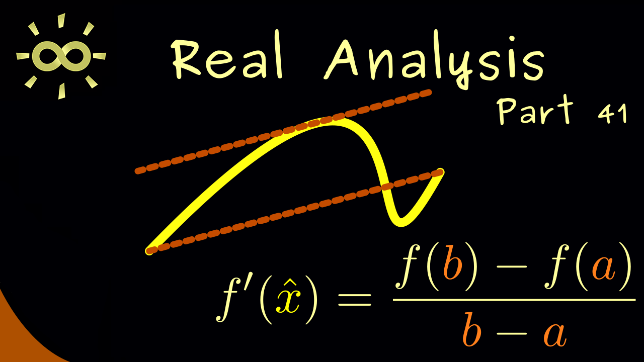
110 00:02:47,470 –> 00:02:48,839 So in dark blue, we have

111 00:02:48,850 –> 00:02:50,500 the function F and light

112 00:02:50,509 –> 00:02:52,100 blue gives us the second.

113 00:02:52,589 –> 00:02:54,199 And now we want to push this

114 00:02:54,210 –> 00:02:56,199 value here to the same level

115 00:02:56,210 –> 00:02:57,220 as this value.

116 00:02:57,869 –> 00:02:59,210 Therefore, in the picture,

117 00:02:59,220 –> 00:03:00,649 this point should go down

118 00:03:00,660 –> 00:03:02,410 exactly by the amount given

119 00:03:02,419 –> 00:03:03,179 by the second.

120 00:03:03,789 –> 00:03:05,410 So you see the overall idea

121 00:03:05,419 –> 00:03:06,869 is simply to subtract the

122 00:03:06,880 –> 00:03:08,270 sequence from the function.

123 00:03:08,919 –> 00:03:10,500 Then the result is that both

124 00:03:10,509 –> 00:03:12,000 points lie at zero

125 00:03:12,509 –> 00:03:13,940 and we have a new function

126 00:03:13,949 –> 00:03:15,289 we can call G.

127 00:03:16,009 –> 00:03:17,029 Now, the important thing

128 00:03:17,039 –> 00:03:18,339 here is that the new function

129 00:03:18,350 –> 00:03:20,270 G is still differentiable

130 00:03:20,279 –> 00:03:21,710 because it’s a difference

131 00:03:21,720 –> 00:03:23,429 of two differential functions.

132 00:03:24,160 –> 00:03:25,460 And moreover, it’s still

133 00:03:25,470 –> 00:03:26,940 defined on the interval.

134 00:03:27,000 –> 00:03:28,830 Ab Now the definition we

135 00:03:28,839 –> 00:03:30,020 described in the picture

136 00:03:30,029 –> 00:03:32,020 is here given in this formula

137 00:03:32,470 –> 00:03:33,970 which is exactly what we

138 00:03:33,979 –> 00:03:34,580 wanted.

139 00:03:34,589 –> 00:03:36,339 The function F minus the

140 00:03:36,350 –> 00:03:36,899 second.

141 00:03:37,589 –> 00:03:38,830 So here we have the constant

142 00:03:38,839 –> 00:03:40,740 slope times X minus a

143 00:03:40,750 –> 00:03:42,740 point A plus F at

144 00:03:42,750 –> 00:03:43,660 this point A.

145 00:03:44,199 –> 00:03:45,770 And of course, here A is

146 00:03:45,779 –> 00:03:47,369 the left bound of the interval.

147 00:03:47,899 –> 00:03:48,169 OK.

148 00:03:48,179 –> 00:03:49,759 Here because G is still

149 00:03:49,770 –> 00:03:51,520 differentiable, we can calculate

150 00:03:51,529 –> 00:03:53,100 the relative, of course,

151 00:03:53,110 –> 00:03:54,339 you can apply the sum rule.

152 00:03:54,350 –> 00:03:55,929 So we have F prime minus

153 00:03:55,940 –> 00:03:57,250 the slope of the second.

154 00:03:57,910 –> 00:03:59,800 So here you see we are already

155 00:03:59,809 –> 00:04:01,539 very close to the mean value

156 00:04:01,550 –> 00:04:02,199 theorem.

157 00:04:02,720 –> 00:04:03,720 Now the only thing that is

158 00:04:03,729 –> 00:04:05,410 left to do here is to apply

159 00:04:05,419 –> 00:04:06,600 Rolle’s theorem.

160 00:04:07,220 –> 00:04:08,699 Please recall before we could

161 00:04:08,710 –> 00:04:09,720 use it in the case that the

162 00:04:09,729 –> 00:04:11,169 left value is equal to the

163 00:04:11,179 –> 00:04:11,899 right value.

164 00:04:11,970 –> 00:04:13,169 And then we found a middle

165 00:04:13,179 –> 00:04:14,600 point such that the derivative

166 00:04:14,610 –> 00:04:15,729 is zero there.

167 00:04:16,170 –> 00:04:17,630 However, now we are in the

168 00:04:17,640 –> 00:04:19,519 case that F of A is not

169 00:04:19,529 –> 00:04:20,700 equal to F of B,

170 00:04:21,140 –> 00:04:22,420 but we shifted the whole

171 00:04:22,429 –> 00:04:24,160 problem such that G

172 00:04:24,170 –> 00:04:25,470 fulfills what we want.

173 00:04:25,890 –> 00:04:26,799 If you don’t believe it,

174 00:04:26,809 –> 00:04:28,320 put A and B into the

175 00:04:28,329 –> 00:04:30,000 definition and you see it

176 00:04:30,429 –> 00:04:32,019 hence, now we can apply Rolle’s

177 00:04:32,220 –> 00:04:33,739 theorem and find a point

178 00:04:33,750 –> 00:04:35,239 X hat where the derivative

179 00:04:35,250 –> 00:04:35,980 is zero.

180 00:04:36,470 –> 00:04:37,980 However, vanishing the relative

181 00:04:37,989 –> 00:04:39,500 for G means that this

182 00:04:39,510 –> 00:04:41,380 expression is equal to zero.

183 00:04:41,779 –> 00:04:43,579 So we simply bring F prime

184 00:04:43,589 –> 00:04:44,589 to the other side.

185 00:04:45,109 –> 00:04:47,010 So not so surprising we found

186 00:04:47,019 –> 00:04:48,700 our mean value theorem.

187 00:04:49,239 –> 00:04:51,019 And indeed this is the whole

188 00:04:51,029 –> 00:04:51,500 proof.

189 00:04:52,170 –> 00:04:52,440 OK.

190 00:04:52,450 –> 00:04:53,769 Then for the end of the video,

191 00:04:53,779 –> 00:04:55,579 let’s look at an application

192 00:04:55,589 –> 00:04:57,079 of this nice theorem.

193 00:04:57,549 –> 00:04:58,970 Again, let’s take a function

194 00:04:58,980 –> 00:05:00,649 F defined on a compact

195 00:05:00,660 –> 00:05:01,179 interval.

196 00:05:01,890 –> 00:05:02,970 And of course, it should

197 00:05:02,980 –> 00:05:04,070 be differential.

198 00:05:04,609 –> 00:05:06,410 Now assume that we know that

199 00:05:06,420 –> 00:05:07,790 the derivative is positive

200 00:05:07,799 –> 00:05:09,089 no matter which point X we

201 00:05:09,100 –> 00:05:09,549 put in.

202 00:05:10,329 –> 00:05:12,140 Then we can look at two arbitrarily

203 00:05:12,149 –> 00:05:14,019 chosen points X one and X

204 00:05:14,029 –> 00:05:16,010 two, where X two is greater

205 00:05:16,019 –> 00:05:17,869 than X one, then we

206 00:05:17,880 –> 00:05:19,049 can apply the mean value

207 00:05:19,059 –> 00:05:20,410 theorem where we shrink the

208 00:05:20,420 –> 00:05:21,980 domain to the interval X

209 00:05:21,989 –> 00:05:22,809 one X two.

210 00:05:23,190 –> 00:05:24,609 This means that we find our

211 00:05:24,619 –> 00:05:26,369 point X hat in the open

212 00:05:26,380 –> 00:05:27,920 interval X one X two.

213 00:05:28,220 –> 00:05:30,070 And as before, at this point,

214 00:05:30,079 –> 00:05:31,589 we find the mean slope,

215 00:05:31,950 –> 00:05:33,679 then we can just multiply

216 00:05:33,690 –> 00:05:35,269 X two minus X one on both

217 00:05:35,279 –> 00:05:36,510 sides and get this

218 00:05:36,519 –> 00:05:37,309 equality.

219 00:05:37,869 –> 00:05:39,450 Now, we can put in our two

220 00:05:39,459 –> 00:05:40,170 assumptions.

221 00:05:40,179 –> 00:05:41,809 First, we know the derivative

222 00:05:41,820 –> 00:05:42,809 is positive.

223 00:05:43,380 –> 00:05:45,079 And secondly, we know X two

224 00:05:45,089 –> 00:05:46,950 minus X one is positive as

225 00:05:46,959 –> 00:05:47,290 well.

226 00:05:47,880 –> 00:05:49,170 Hence, we can conclude the

227 00:05:49,179 –> 00:05:50,890 left hand side of the equality

228 00:05:50,899 –> 00:05:52,410 is also positive,

229 00:05:52,799 –> 00:05:54,359 which means the value

230 00:05:54,369 –> 00:05:56,160 FX two is greater than the

231 00:05:56,170 –> 00:05:57,480 value FX one.

232 00:05:57,829 –> 00:05:59,239 And since the numbers X one

233 00:05:59,250 –> 00:06:01,200 X two were arbitrarily chosen,

234 00:06:01,209 –> 00:06:02,559 we conclude that the function

235 00:06:02,570 –> 00:06:04,420 F is increasing or

236 00:06:04,429 –> 00:06:05,459 more concretely, we would

237 00:06:05,470 –> 00:06:06,859 say F is strictly

238 00:06:06,869 –> 00:06:08,579 monotonically increasing.

239 00:06:09,000 –> 00:06:10,619 Now, indeed, this is a nice

240 00:06:10,630 –> 00:06:11,160 result.

241 00:06:11,170 –> 00:06:12,510 We merely get out of the

242 00:06:12,519 –> 00:06:13,980 mean value theorem.

243 00:06:14,250 –> 00:06:15,510 So in short, we can simply

244 00:06:15,519 –> 00:06:17,070 say if the derivative is

245 00:06:17,079 –> 00:06:18,679 always positive, we get out

246 00:06:18,690 –> 00:06:19,910 a function that is at all

247 00:06:19,920 –> 00:06:21,660 points increasing strictly

248 00:06:21,670 –> 00:06:22,670 monotonically.

249 00:06:23,089 –> 00:06:24,359 And of course, with a similar

250 00:06:24,369 –> 00:06:25,940 proof, we can also look at

251 00:06:25,950 –> 00:06:27,829 cases with a negative derivative.

252 00:06:28,459 –> 00:06:29,750 This case might not surprise

253 00:06:29,760 –> 00:06:30,029 you.

254 00:06:30,040 –> 00:06:31,309 We simply get out that the

255 00:06:31,320 –> 00:06:33,070 function is strictly monotonically

256 00:06:33,079 –> 00:06:33,760 decreasing.

257 00:06:33,769 –> 00:06:35,709 Then in addition, we can

258 00:06:35,720 –> 00:06:37,239 also look at the cases where

259 00:06:37,250 –> 00:06:38,380 we don’t have the strict

260 00:06:38,390 –> 00:06:39,200 inequality.

261 00:06:39,649 –> 00:06:40,970 This means if you look at

262 00:06:40,980 –> 00:06:42,640 the proof, we will also lose

263 00:06:42,649 –> 00:06:44,239 the strict inequality here.

264 00:06:44,760 –> 00:06:46,119 Otherwise the proof works

265 00:06:46,130 –> 00:06:47,309 exactly the same.

266 00:06:47,679 –> 00:06:49,049 However, since we lose the

267 00:06:49,059 –> 00:06:50,119 strict inequality.

268 00:06:50,130 –> 00:06:51,339 We just have functions that

269 00:06:51,350 –> 00:06:52,940 are monotonically increasing

270 00:06:52,950 –> 00:06:54,049 or decreasing.

271 00:06:54,649 –> 00:06:54,869 OK.

272 00:06:54,880 –> 00:06:55,980 With this, we now have a

273 00:06:55,989 –> 00:06:57,380 common application for

274 00:06:57,390 –> 00:06:59,130 derivatives when we want to analyze

275 00:06:59,140 –> 00:06:59,920 functions.

276 00:07:00,299 –> 00:07:01,369 And of course, this will

277 00:07:01,380 –> 00:07:03,220 come in handy a lot later.

278 00:07:03,899 –> 00:07:05,239 Therefore, I really hope

279 00:07:05,250 –> 00:07:07,140 I see you in later videos.

280 00:07:07,720 –> 00:07:09,519 Have a nice day and bye.

Q1: Let $f \colon [a,b] \rightarrow \mathbb{R}$ be a differentiable function. What is the correct formulation for the mean value theorem?

A1: There is $\hat{x}$ with $f^\prime(\hat{x}) = 0$.

A2: There is $\hat{x}$ with $f^\prime(\hat{x}) = f(a)$.

A3: There is $\hat{x}$ with $f^\prime(\hat{x}) = \frac{f(b) - f(a)}{b - a}$.

A4: There is $\hat{x}$ with $f^\prime(\hat{x}) = (f(b) - f(a) ) \cdot (b-a)$.

Q2: Let $f \colon [a,b] \rightarrow \mathbb{R}$ be a differentiable function with $ f^\prime(x) > 0$ for all $x$. What does the mean value theorem imply?

A1: $f$ is constant.

A2: $f$ has a local maximum at $a$.

A3: $f$ is strictly monotonically increasing.

A4: $f$ is strictly monotonically decreasing.

Q3: Let $f \colon [a,b] \rightarrow \mathbb{R}$ be a differentiable function with $ f^\prime(x) \leq 0$ for all $x$. What does the mean value theorem imply?

A1: $f$ is constant.

A2: $f$ has a local maximum at $b$.

A3: $f$ monotonically increasing.

A4: $f$ monotonically decreasing.