Hello and welcome to my ongoing video course about Partial Differential Equations, already consisting of 25 videos. The video series is called Partial Differential Equations (PDEs). The course it’s not finished yet. This course builds on the foundation laid in the Ordinary Differential Equations (ODEs) series, expanding into the more complex and multi-dimensional world of PDEs. Alongside the videos, you’ll find additional text explanations to help reinforce the material. To test your knowledge, use the quizzes, and refer to the PDF versions of the lessons whenever needed. If you have any questions, feel free to participate in the community discussion forum. Without further ado, let’s get started!
Part 1 - Introduction and Definition
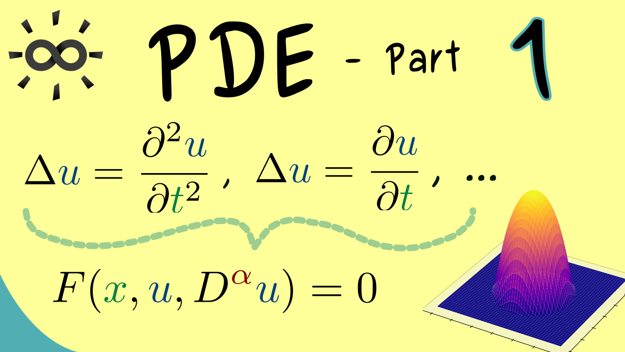
Let’s start the video series with some basic notions we will use throughout the course. For example, we have to know what we mean by a partial differential equation and a classical solution of it.
Part 2 - Laplace’s Equation
One of the most important partial differential equations is Laplace’s equation where the solutions are called harmonic fucntions. We will try to find solutions that respect the radial symmetry because these can be used a base for the construcion of other solutions.

Part 3 - Fundamental Solution of Laplace’s Equation
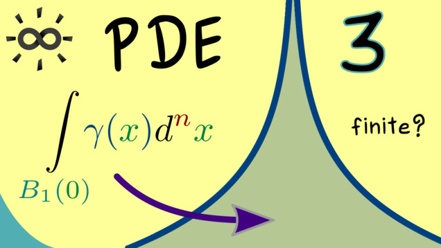
The fundamental solution for Laplace’s equation is sometimes also called Newtonian kernel because of its application in physics. Indeed, in three dimensions, we have $\gamma(x) = \frac{1}{4 \pi} \frac{1}{\| x \|}$ for the fundamental solution. Obviously, there is a singularity at the origin, but it turns out that inside an integral it is no problem at all. Let’s show that for an arbitrary dimension $n$ as well.
Part 4 - Mean-Value Property of Harmonic Functions
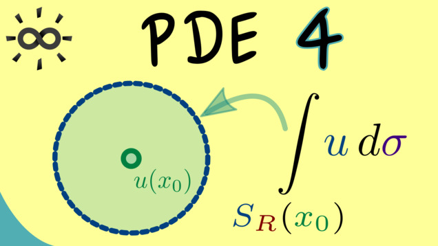
The solutions of Laplace’s equation have some nice properties that can be surpring. For example, we can show that the values of the function at a point is already determined by the values of the function on a sphere around this point. This is what we mean by the mean-value property of a function. Let’s prove this by using Green’s identity and the fact that we can move a derivative inside the integral under our assumptions here.
Other videos related to this topic:
- Multidimensional Integration 9 | Integration with Polar Coordinates
- Multidimensional Integration 11 | Green’s Identities
- Measure Theory 10 | Lebesgue’s Dominated Convergence Theorem
- Multidimensional Integration 12 | Differentiation Under The Integral Sign
Part 5 - Maximum Principle for Harmonic Functions
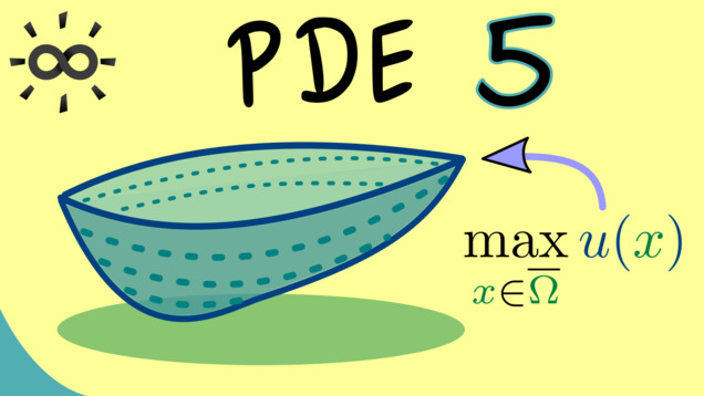
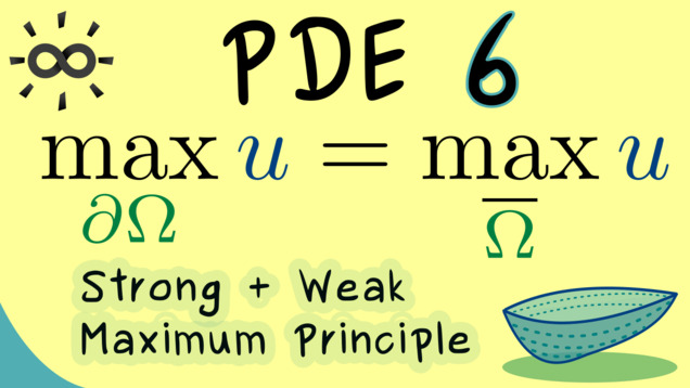
A direct consequence of the mean-value property of harmonic functions is the so-called maximum principle. It roughly says that the maximum of any harmonic function $u : \Omega \rightarrow \mathbb{R}$ is always found on the boundary $\partial \Omega$. We can even distiguish a strong and weak maximum principle depending if we have a connected set $\Omega$ or not.
Other videos related to this topic:
Part 6 - Proof of Maximum Principle
Let’s prove the two statements from the last video. We will need some topology knowledge for connected sets, which you can find in the Basic Topology course. In particular, we can use from there that path-connected sets are also connected. Therefore, we will first show the strong maximum principle and use it to prove the weak maximum principle.
Other videos related to this topic:
Part 7 - Uniqueness of the Boundary Value Problem for Poisson’s Equation
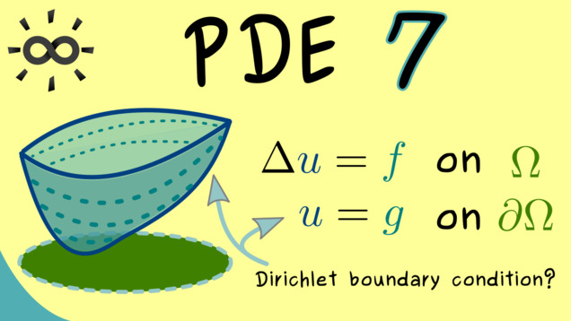
We can generalize our the important PDE given by Laplace’s equation to Poisson’s equation by changing the right-hand side to a continuous function $f$. So we search for functions $u$ where the Laplacian $\Delta u$ is given by $f$ on the whole open domain $\Omega$. Now, if we also claim that $u$ should be equal to a continuous function $g$ on the boundary $\partial \Omega$, then we speak of a boundary-value problem. In particular, in this case, we have so-called Dirichlet boundary conditions. It turns out that such a boundary-value problem on a bounded set $\Omega$ has at most one solution, so we definitely have uniqueness if a solution exists. As we will show in the video, this property immediately follows from the maximum principle for harmonic functions.
Part 8 - Standard Mollifier
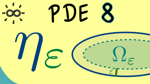
In the following, we will discuss a common tool in analysis known as the standard mollifier, which can be used to smoothen continuous functions. One uses an exponential functions to define a $C^\infty$-function with compact support. By scaling it appropriately, we get a so-called Dirac sequence that can be used to approximate the original function. Let’s discuss how that works in detail for a function $u : \Omega \rightarrow \mathbb{R}$, where $\Omega$ is an open set in $\mathbb{R}^n$.
Other videos related to this topic:
- An Approximation Theorem for Continuous Functions
- Multidimensional Integration 12 | Differentiation Under The Integral Sign
Part 9 - Regularity of Harmonic Functions
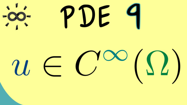
The next topic about regularity means that the solutions of Laplace’s equation are much smoother than what the formal equation requires. Instead of $C^2$-functions, we actually get $C^\infty$-functions out.
Other videos related to this topic:
Part 10 - Liouville’s Theorem for Harmonic Functions
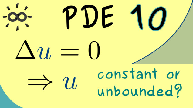
You might already know Liouville’s theorem for holomorphic functions from Complex Analysis. In fact, the following discussion is a generalization of this result. We will show that every harmonic function defined on the whole space $\mathbb{R}^n$ is either constant or unbounded. The key ingredient for the proof is to have an estimate for the partial derivatives of a harmonic function defined on a ball.
Other videos related to this topic:
- Multidimensional Integration 9 | Integration with Polar Coordinates
- Multidimensional Integration 11 | Green’s Identities
Part 11 - Normal Derivative of Newtonian Kernel
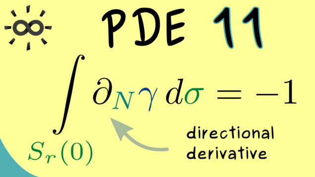
Our goal is to solve Poisson’s equation $\Delta u = f$ for a given function $f$. It will turn out that the fundamental solution of Laplace’s equation, denoted by $\gamma$ plays the key role there. However, in order to use it correctly, we first have to check some properties of it. Let’s start with the normal derivative of $\gamma$ at the sphere.
Other videos related to this topic:
- Multidimensional Integration 12 | Differentiation Under The Integral Sign
- Multidimensional Integration 11 | Green’s Identities
Part 12 - Properties of Newtonian Kernel
We can easily extend the result from the last video to get a property that looks like something we could call delta function. It just means that in a limit process of an integral, we get the value of a function at a given point. This is a nice property of the normal derivative on the sphere and we will use it to find a representation formula for general $C^2$-functions that could be used to solve Poisson’s equation. But let’s first prove this property.

Part 13 - Representation Formula for Poisson’s Equation
The following representation formula that holds for any $C^2$-functions $u$ is quite interesting. The singularity of $\gamma$ allows to write each value $u(x_0)$ as a combination of a surface integral with a volume integral as long as the point $x_0$ lies inside the domain of the volume integral. Furthermore, for harmonic functions, this representation formula becomes even shorter.

Other videos related to this topic:
Part 14 - Newtonian Potential
In this video, we will finally construct a solution of Poisson’s equation. We can do it by using the convolution with the fundamental solution of Laplace’s equation. This function $\gamma \ast f$ is often called Newtonian potential because of the historical usage of the gravitational potential. However, it also occurs as the Coulomb potential in electrostatics. We will also show that this solution of Poisson’s equation is unique if we assume that the solution vanishes at infinity.

Other videos related to this topic:
Part 15 - Green’s Function
Let’s go back to the boundary-value problem for Poisson’s equation with Dirichlet boundary conditions. This means that we have two continuous functions $f$ and $g$, where $f$ is on the right of Poisson’s equation and $g$ should give the boundary values of the solution. It turns out that our representation formula for $C^2$-functions almost already catches that problem. We just have get rid of the normal derivative of the solution. This is what can be done by Green’s function, which we can define for every open subset $\Omega \subseteq \mathbb{R}^n$.

Other videos related to this topic:
Part 16 - Symmetry Property of Green’s Function
Let’s look at Green’s function more closely. The definition is completely different in the two variables $x$ and $y$ in the function $G(x,y)$. However, we can still show that we the function is symmetric if we concentrate on points in $\Omega$ that don’t coincide. The proof is similar to the proof of the representation formulas we have done before.

Other videos related to this topic:
- Multidimensional Integration 11 | Green’s Identities
- Partial Differential Equations 12 | Properties of Newtonian Kernel
Part 17 - Green’s Function for Unit Ball
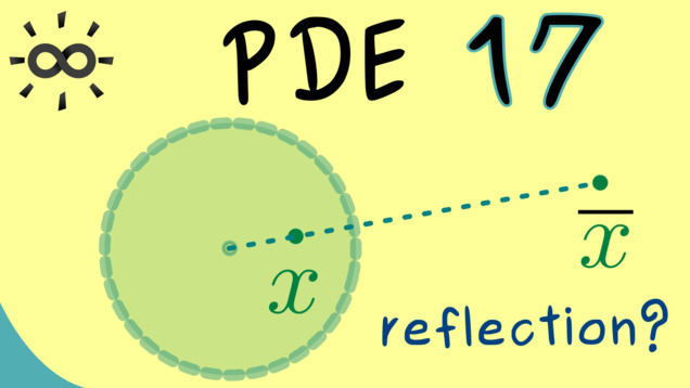
As an explicit and important example of Green’s function, let’s consider the unit ball in $\mathbb{R}^n$. It turns out that we easily define it by using a reflection with respect to the unit sphere.
Part 18 - Poisson’s Integral Formula for Unit Ball
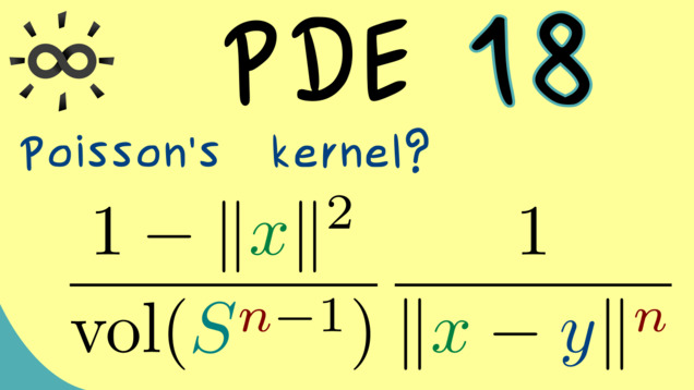
By using Green’s function for the ball from the last video, we can actually formulate a solution formula for the boundary value problem. For Laplace’s equation, this one is known as Poisson’s integral formula and corresponding integrand is the so-called Poisson kernel.
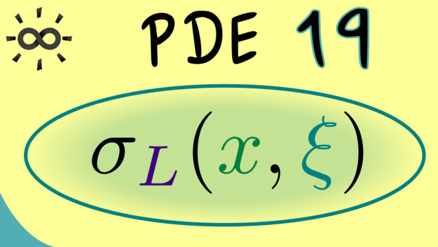
Part 19 - Elliptic Differential Operators
The Laplacian is the typical example of a so-called elliptic operator. Let’s explain where this name comes from and let’s also look at so-called parabolic and hyperpolic PDEs. We can sketch some examples in two-dimensions.
Other videos related to this topic:
- Abstract Linear Algebra 47 | Spectral Theorem for Normal Matrices
- Multivariable Calculus 15 | Multi-Index Notation
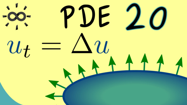
Part 20 - Heat Equation - Motivation
As already mentioned in the last video, we want to start discussing the prime example of a parabolic PDE. This is the so-called heat equation or diffussion equation. It defined for a function with $n+1$ variables, where we can always interpret one variable as the time variable and denote it by $t$. You can already remember that this time variable is special because we only have a first order partial derivative for it. However, before discussing the mathematical content of the heat equation, let’s first see why it often naturally occurs in application. It’s just a result of a conservation law of a quantity and a linear relation between flux and gradient of this aforementioned quantity. Let’s see what this actually means.
Other videos related to this topic:
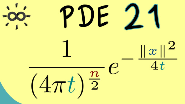
Part 21 - Heat Kernel - Definition
Using the same approach as for Laplace’s equation, we want to construct a fundamental solution of the heat equation. We will always call it the heat kernel and denote it by $\Phi(x,t)$. It’s given by an exponential function that combines space variables and time variables. But before we talk about the properties, let’s use some symmetry arguments to justify why we even get an exponential function as a possible solution of the heat equation.
Other videos related to this topic:
- Ordinary Differential Equations 7 | Solving Linear Equations of First Order
- Distributions 25 | Heat Equation with Fourier Transform
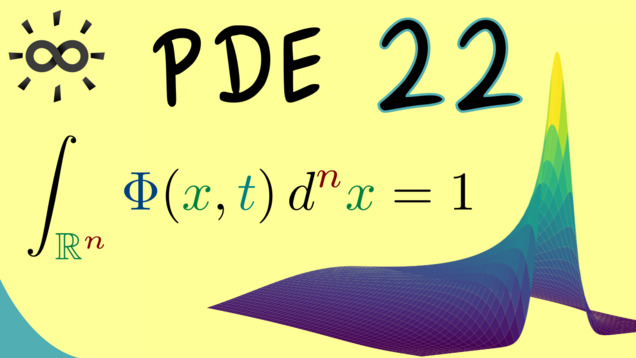
Part 22 - Heat Kernel - Properties
The heat kernel should act in a similar way to the heat equation as the Newtonian kernel acts to Laplace’s equation. Let’s start with a normalization property. This means that for any time $t>0$, the integral of $\Phi(\cdot, t)$, taking over the whole space $\mathbb{R}^n$ is equal to 1. Let’s prove it!
Other videos related to this topic:
- Multidimensional Integration 3 | Fubini’s Theorem
- Fourier Transform 30 | Fixed Point of Fourier Integral Transform
Part 23 - Heat Equation - Initial Value Problem
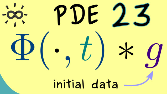
The power of the fundamental solution of the heat equation lies in the fact that we can easily construct more solutions by using the convolution with a bounded continuous function $g$ on $\mathbb{R}^n$. Then it turns out that this a solution of the initial value problem with initial data given by $g$. In order to prove this, we will need so-called Dirac sequences and an approximation theorem for continuous functions.
Other videos related to this topic:
- Multidimensional Integration 12 | Differentiation Under The Integral Sign
- An Approximation Theorem for Continuous Functions
Part 24 - Maximum Principle for Heat Equation
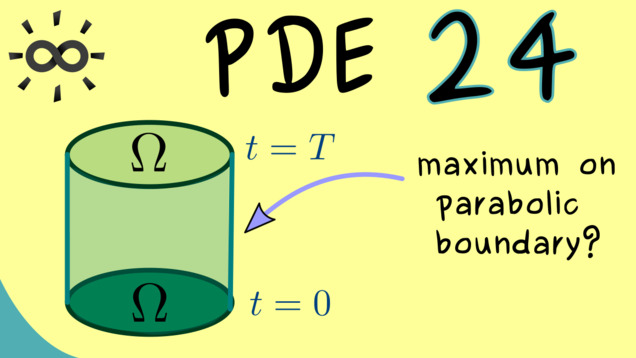
We have only discussed the existence of a solution for the initial value problem before. We didn’t say anything about uniqueness yet. The reason for that is that we need the maximum principle to show uniqueness. The maximum principle for the heat equation is similar to the one for Laplace’s equation, which means that the maximum of a solution is always attained on the boundary. However, in the case of the heat equation, the corresponding boundary is a special one and called the parabolic boundary.
Part 25 - Proof of Maximum Principle for Heat Equation
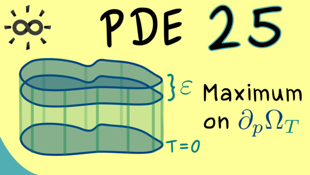
Let’s prove the statement from the last video by using some Multivariable Calculus and Linear Algebra knowledge.
Other videos related to this topic:
- Multivariable Calculus 18 | Local Extrema
- Multivariable Calculus 20 | Sylvester’s Criterion
- Tensor Analysis 9 | Trace and Contraction
Connections to other courses
Summary of the course Partial Differential Equations
-
You can download the whole PDF here and the whole dark PDF.
-
You can download the whole printable PDF here.
- Ask your questions in the community forum about Partial Differential Equations.
Ad-free version available:
Click to watch the series on Vimeo.