-
Title: Introduction and Definition
-
Series: Partial Differential Equations
-
Chapter: Introduction
-
YouTube-Title: Partial Differential Equations 1 | Introduction and Definition
-
Bright video: Watch on YouTube
-
Dark video: Watch on YouTube
-
Ad-free video: Watch Vimeo video
-
Forum: Ask a question in Mattermost
-
Dark-PDF: Download PDF version of the dark video
-
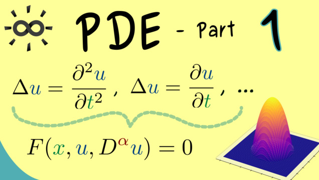
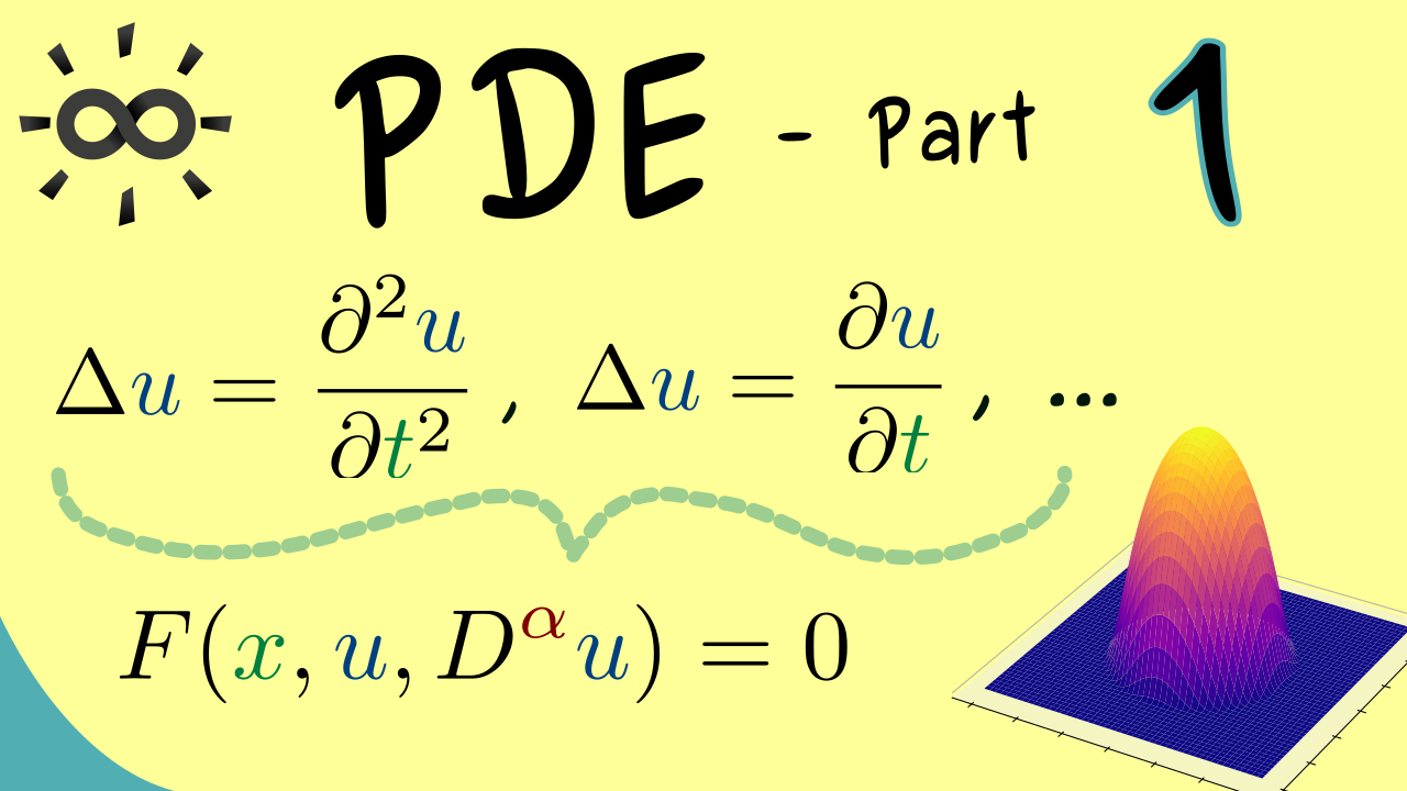
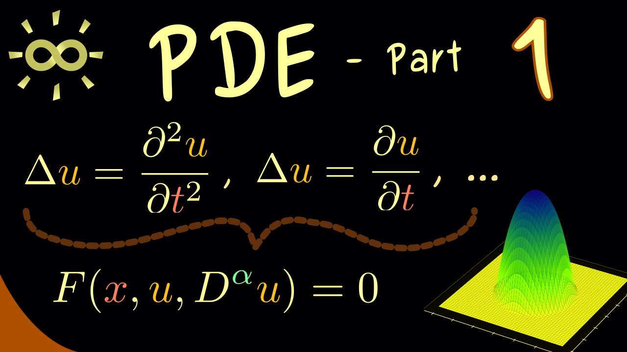
Print-PDF: Download printable PDF version
-
Thumbnail (bright): Download PNG
-
Thumbnail (dark): Download PNG
-
Subtitle on GitHub: pde01_sub_eng.srt
-
Download bright video: Link on Vimeo
-
Timestamps (n/a)
-
Subtitle in English
1 00:00:00.735 –> 00:00:03.685 Hello and welcome to Partial Differential Equations,
2 00:00:04.025 –> 00:00:07.005 the new video series where I want to talk about the theory
3 00:00:07.345 –> 00:00:09.045 of partial differential equations.
4 00:00:09.705 –> 00:00:13.125 And I can already tell you this topic is often abbreviated
5 00:00:13.265 –> 00:00:14.805 to just PDE.
6 00:00:15.385 –> 00:00:16.605 We will also do this here.
7 00:00:16.825 –> 00:00:19.725 And moreover, since this is a really huge subject,
8 00:00:20.305 –> 00:00:23.005 you can expect a lot of videos in this series.
9 00:00:23.575 –> 00:00:26.705 However, before I start telling you what we will cover here,
10 00:00:27.065 –> 00:00:28.945 I first want to thank all the nice people
11 00:00:28.965 –> 00:00:30.865 who support the channel on Steady, here on
12 00:00:30.865 –> 00:00:32.145 YouTube, or via other means.
13 00:00:32.935 –> 00:00:34.915 And please don’t forget that you can download a lot
14 00:00:34.915 –> 00:00:37.835 of additional material with the link in the description.
15 00:00:38.455 –> 00:00:39.995 And now without further ado,
16 00:00:40.205 –> 00:00:42.475 let’s immediately jump into the description
17 00:00:42.495 –> 00:00:43.755 of this video course.
18 00:00:44.655 –> 00:00:46.155 We will do a classical approach
19 00:00:46.415 –> 00:00:49.955 by first discussing the three most important examples
20 00:00:49.955 –> 00:00:51.555 of partial differential equations.
21 00:00:52.235 –> 00:00:55.055 All of these will include the famous Laplace operator,
22 00:00:55.685 –> 00:00:59.695 also often called Laplacian denoted by a capital delta.
23 00:01:00.445 –> 00:01:03.225 And the first PDE here is just Laplace’s equation
24 00:01:03.395 –> 00:01:06.505 where we just search for solutions for the Laplacian.
25 00:01:07.335 –> 00:01:08.985 This will be already interesting
26 00:01:09.125 –> 00:01:11.545 and of course I will explain more about the partial
27 00:01:11.905 –> 00:01:13.705 derivatives that go into this equation.
28 00:01:14.605 –> 00:01:17.665 And then the second PDE is the so-called heat equation
29 00:01:17.795 –> 00:01:19.705 where we also have the Laplacian,
30 00:01:20.325 –> 00:01:23.865 but also first order partial derivative with respect
31 00:01:23.885 –> 00:01:25.345 to a time variable T.
32 00:01:26.055 –> 00:01:29.155 So you already see this is a different kind of PDE,
33 00:01:29.415 –> 00:01:32.475 and it has a lot of applications as the name suggests.
34 00:01:33.275 –> 00:01:36.735 And in that sense, the third type also has it in its name.
35 00:01:37.005 –> 00:01:38.815 It’s the so-called wave equation.
36 00:01:39.515 –> 00:01:41.895 And this one also has a right hand side given
37 00:01:42.035 –> 00:01:44.895 by a partial derivative, but now of second order.
38 00:01:45.475 –> 00:01:47.175 So the three equations look similar,
39 00:01:47.555 –> 00:01:50.295 but these details here completely changed their behavior.
40 00:01:51.195 –> 00:01:54.175 And because of that, one has some special names in the
41 00:01:54.175 –> 00:01:58.385 theory of PDEs, the wave equation is a hyperbolic one,
42 00:01:58.385 –> 00:02:01.345 whereas the heat equation is a parabolic one.
43 00:02:01.965 –> 00:02:04.545 And finally, Laplace’s equation is a
44 00:02:04.545 –> 00:02:05.985 so-called elliptic one.
45 00:02:06.725 –> 00:02:10.545 So the overall idea here is if you understand these explicit
46 00:02:10.825 –> 00:02:14.825 examples of PDEs, you can lift these to the general cases.
47 00:02:15.525 –> 00:02:17.905 And indeed this is something we will do afterwards
48 00:02:18.275 –> 00:02:20.825 after our discussion of these three types.
49 00:02:21.655 –> 00:02:24.065 This will be a more general abstract theory
50 00:02:24.435 –> 00:02:27.465 where we talk about Sobolev spaces, distributions and so on.
51 00:02:28.005 –> 00:02:30.505 But this is definitely something I will do later
52 00:02:30.925 –> 00:02:33.865 and maybe I put some stuff into separate series,
53 00:02:33.865 –> 00:02:36.105 like I’ve already done it for the distributions.
54 00:02:37.125 –> 00:02:38.685 Speaking of that, I should definitely tell
55 00:02:38.685 –> 00:02:39.725 you the requirements,
56 00:02:39.865 –> 00:02:42.045 the other parts of mathematics you need
57 00:02:42.265 –> 00:02:44.525 to understand this video series here.
58 00:02:44.985 –> 00:02:47.405 So let’s put the PDE course here in the middle
59 00:02:47.745 –> 00:02:50.245 and then I tell you which other series
60 00:02:50.385 –> 00:02:51.565 you should watch before that.
61 00:02:52.305 –> 00:02:55.325 In fact, the most important requirement is the multivariable
62 00:02:55.765 –> 00:02:58.565 calculus course because there we defined partial
63 00:02:59.005 –> 00:03:02.925 derivatives and obviously a PDE has partial derivatives
64 00:03:03.105 –> 00:03:04.325 as the main ingredient.
65 00:03:05.385 –> 00:03:07.685 If not, we only would have an ODE,
66 00:03:07.985 –> 00:03:09.845 an ordinary differential equation.
67 00:03:10.545 –> 00:03:13.165 And of course it makes sense to first learn about this case
68 00:03:13.305 –> 00:03:16.085 before you go to the partial differential equations.
69 00:03:16.865 –> 00:03:19.845 In addition to that, I also would say it’s important
70 00:03:19.875 –> 00:03:22.725 that you know how to integrate in higher dimensions,
71 00:03:23.345 –> 00:03:24.645 and for that it’s sufficient
72 00:03:24.645 –> 00:03:27.325 that you know my multi-dimensional integration course.
73 00:03:28.175 –> 00:03:31.115 You might know that I also have a measure theory course
74 00:03:31.215 –> 00:03:32.955 for the general theory of integration,
75 00:03:33.135 –> 00:03:36.115 but it’s not really necessary for our PDE course.
76 00:03:36.885 –> 00:03:39.515 Still, there are some connections between the two series
77 00:03:39.515 –> 00:03:43.255 that might help you, but it’s not really necessary. The same,
78 00:03:43.335 –> 00:03:45.455 I would say for the functional analysis course.
79 00:03:45.845 –> 00:03:48.135 It’s good to know some operator theory,
80 00:03:48.515 –> 00:03:49.775 but it’s not really needed.
81 00:03:50.555 –> 00:03:51.575 Indeed, this is something
82 00:03:51.575 –> 00:03:54.295 that we might need in the end when we go
83 00:03:54.295 –> 00:03:56.895 to the abstract theory and talk about Sobolev spaces.
84 00:03:57.745 –> 00:04:01.205 So you see my idea here is to assume not too much such
85 00:04:01.205 –> 00:04:03.685 that I can explain everything at the spot
86 00:04:03.985 –> 00:04:05.645 inside the series when we need it.
87 00:04:06.465 –> 00:04:09.235 Okay. So with that out of the way, we can immediately go
88 00:04:09.235 –> 00:04:11.715 to the first definition to answer the question,
89 00:04:12.065 –> 00:04:13.475 what is the PDE?
90 00:04:14.105 –> 00:04:16.115 This definition is quite easy to explain
91 00:04:16.145 –> 00:04:17.835 because we already know
92 00:04:17.835 –> 00:04:19.995 that partial derivatives should play a role.
93 00:04:20.655 –> 00:04:23.835 And these partial derivatives come from an unknown function
94 00:04:24.135 –> 00:04:27.635 we call u and domain of u we call Omega,
95 00:04:27.895 –> 00:04:30.275 and it’s usually an open set in Rn.
96 00:04:30.865 –> 00:04:34.115 Otherwise, the values of u should be a real numbers.
97 00:04:34.895 –> 00:04:38.995 So now please remember Omega is definitely a subset in Rn
98 00:04:39.295 –> 00:04:40.355 and usually open.
99 00:04:41.205 –> 00:04:43.705 In fact, in a lot of cases we want to have even more.
100 00:04:44.045 –> 00:04:46.625 For example, it’s usually also connected.
101 00:04:47.075 –> 00:04:49.925 However, this is something we will talk about later here.
102 00:04:49.925 –> 00:04:52.165 Just remember that we have an open set
103 00:04:52.425 –> 00:04:53.805 and the dimension is greater
104 00:04:53.825 –> 00:04:57.935 or equal than two. Obviously here, if n was equal to one,
105 00:04:58.155 –> 00:05:00.855 we would be in our ordinary differential equations case.
106 00:05:00.855 –> 00:05:03.395 Again, let’s finish this definition.
107 00:05:03.535 –> 00:05:06.115 So we have an equation where partial derivatives
108 00:05:06.115 –> 00:05:07.275 of u are involved.
109 00:05:08.095 –> 00:05:09.675 So more formally we could write
110 00:05:09.755 –> 00:05:11.755 that we have a function capital F,
111 00:05:12.375 –> 00:05:15.555 and then the first input is a point x from Omega.
112 00:05:15.905 –> 00:05:18.355 Then the second input is our function u,
113 00:05:18.975 –> 00:05:21.075 and then all the other inputs are given
114 00:05:21.215 –> 00:05:22.515 by partial derivatives.
115 00:05:23.145 –> 00:05:25.125 And there you know, these can always be written
116 00:05:25.125 –> 00:05:26.885 with a multi-index alpha.
117 00:05:27.065 –> 00:05:30.445 So we have D alpha u for a partial derivative,
118 00:05:30.945 –> 00:05:34.485 and then obviously all possible multi-indices could go in,
119 00:05:34.665 –> 00:05:36.605 but there’s definitely a highest order
120 00:05:36.905 –> 00:05:38.405 and we call this one m.
121 00:05:38.945 –> 00:05:42.605 So for explicit examples, we can choose a minimal m here,
122 00:05:42.745 –> 00:05:45.565 and this will be the order of our PDE.
123 00:05:46.105 –> 00:05:48.765 And of course we can always write this equation such
124 00:05:48.765 –> 00:05:50.885 that we have a zero on the right hand side.
125 00:05:51.615 –> 00:05:54.595 So this formulation already explains what a PDE is,
126 00:05:54.895 –> 00:05:56.835 but to make it more precise, we should
127 00:05:57.405 –> 00:05:59.765 evaluate all these functions at the point x.
128 00:06:00.395 –> 00:06:02.685 This means we have u of x here
129 00:06:02.985 –> 00:06:05.765 and all the partial derivatives of x as well.
130 00:06:06.505 –> 00:06:09.275 With that, our capital F is now a well-defined map,
131 00:06:09.325 –> 00:06:13.075 which gets omega as an input here, R as an input there.
132 00:06:13.335 –> 00:06:16.315 And a lot of Cartesian products of R there.
133 00:06:17.215 –> 00:06:19.075 Of course, this is just a formal description
134 00:06:19.075 –> 00:06:21.715 and what we actually mean you immediately see in an example.
135 00:06:22.535 –> 00:06:25.435 So for example, we could say we have the sine function
136 00:06:25.435 –> 00:06:27.075 where u of x goes in
137 00:06:27.815 –> 00:06:30.915 and then maybe we add the first partial derivative of u
138 00:06:30.985 –> 00:06:33.355 with respect to x1,
139 00:06:34.285 –> 00:06:36.305 and then maybe we multiply this
140 00:06:36.415 –> 00:06:39.225 with the second order partial derivative of u.
141 00:06:39.805 –> 00:06:43.505 And this one should be with respect to x1 and x2.
142 00:06:44.425 –> 00:06:48.085 And as before, everything here is evaluated at the point x.
143 00:06:48.855 –> 00:06:52.075 And there you see the highest order for the partial derivatives,
144 00:06:52.225 –> 00:06:55.835 this m that is involved here could be chosen as two.
145 00:06:56.565 –> 00:06:59.425 So this is the minimal choice for our m and
146 00:06:59.425 –> 00:07:03.025 therefore we say that this PDE has order two.
147 00:07:03.645 –> 00:07:06.465 So just means that the highest order of partial derivatives
148 00:07:06.495 –> 00:07:08.505 that is involved is of order two.
149 00:07:09.415 –> 00:07:11.515 So maybe let’s look at a very general example
150 00:07:11.685 –> 00:07:13.795 where D alpha u is involved.
151 00:07:14.605 –> 00:07:18.105 And now we could say we sum them up, up to order m.
152 00:07:18.845 –> 00:07:22.065 And what we get then is a PDE of order m.
153 00:07:22.285 –> 00:07:24.985 And we would also say it’s a linear PDE.
154 00:07:25.565 –> 00:07:29.065 It is called linear because all the partial derivatives go
155 00:07:29.095 –> 00:07:31.385 into the equation in a linear sense.
156 00:07:32.145 –> 00:07:35.485 And please note also the function u goes in linearly
157 00:07:35.635 –> 00:07:38.845 because it corresponds to the multi-index just given
158 00:07:38.945 –> 00:07:41.485 by zeros, which also tells me
159 00:07:41.555 –> 00:07:43.245 that in a general description here,
160 00:07:43.465 –> 00:07:46.485 we should actually exclude this case in the third part.
161 00:07:47.545 –> 00:07:50.635 Okay? But now the term linear also allows
162 00:07:50.695 –> 00:07:52.195 for coefficients in front.
163 00:07:52.965 –> 00:07:55.385 So if you want, we could just take functions a
164 00:07:55.575 –> 00:07:56.825 with index alpha.
165 00:07:57.485 –> 00:08:00.225 So multiplying with functions that depend on x
166 00:08:00.245 –> 00:08:01.825 but not on u is allowed.
167 00:08:02.305 –> 00:08:03.625 Moreover, this is actually
168 00:08:03.625 –> 00:08:06.265 what we would call a homogeneous linear PDE.
169 00:08:06.445 –> 00:08:09.065 So we can also make it inhomogeneous,
170 00:08:09.755 –> 00:08:12.585 which means we could have a function f on the right as well.
171 00:08:13.265 –> 00:08:14.995 Obviously for the general description,
172 00:08:14.995 –> 00:08:16.435 we could just subtract this
173 00:08:16.535 –> 00:08:18.755 to still have a zero on the right hand side.
174 00:08:18.975 –> 00:08:22.075 But for a linear PDE, this is a common choice to write it.
175 00:08:22.655 –> 00:08:24.715 And in fact, you can see this as a definition.
176 00:08:24.865 –> 00:08:28.075 This is exactly what we call a linear PDE.
177 00:08:28.625 –> 00:08:31.325 And now for the last definition of this video, I want
178 00:08:31.325 –> 00:08:34.045 to tell you what a solution of a PDE is.
179 00:08:34.915 –> 00:08:37.895 In fact, what we have here at the start is a so-called
180 00:08:37.965 –> 00:08:39.095 classical solution.
181 00:08:39.715 –> 00:08:41.055 So you might already see here
182 00:08:41.055 –> 00:08:44.975 that later in this course we will also define other solution
183 00:08:45.135 –> 00:08:48.175 notions, why these other notions will be helpful,
184 00:08:48.435 –> 00:08:51.095 we will see later. But first, let’s stay
185 00:08:51.095 –> 00:08:52.255 with the classical term.
186 00:08:53.055 –> 00:08:55.285 And indeed this term is not complicated at all
187 00:08:55.315 –> 00:08:56.645 because it’s just given
188 00:08:56.785 –> 00:09:00.365 by a function u defined on the whole set Omega.
189 00:09:01.145 –> 00:09:04.045 And moreover, we need that all the partial derivatives
190 00:09:04.145 –> 00:09:07.925 of u that are involved in the PDE are well-defined.
191 00:09:08.505 –> 00:09:09.605 So the best case would be
192 00:09:09.605 –> 00:09:11.325 that we have partial differentiability
193 00:09:11.865 –> 00:09:13.685 for all the orders we need.
194 00:09:14.265 –> 00:09:16.965 So in any case, if everything here is well-defined,
195 00:09:17.185 –> 00:09:19.725 we can put this stuff into our PDE
196 00:09:20.265 –> 00:09:22.445 and then we just have the pointwise equality
197 00:09:22.985 –> 00:09:24.685 for every x in Omega.
198 00:09:25.465 –> 00:09:27.205 So you see this totally makes sense
199 00:09:27.425 –> 00:09:28.885 for every point x you want
200 00:09:28.885 –> 00:09:31.365 to put in the equation should be satisfied.
201 00:09:32.025 –> 00:09:33.925 And this makes it a classical solution,
202 00:09:34.225 –> 00:09:36.525 as you might already know it from the ordinary
203 00:09:36.525 –> 00:09:37.645 differential equations.
204 00:09:38.345 –> 00:09:40.565 And for now, we will keep this solution term,
205 00:09:40.785 –> 00:09:41.845 but please keep in mind
206 00:09:41.995 –> 00:09:44.405 that other solution notions also exist.
207 00:09:45.075 –> 00:09:46.655 But this is definitely something for the future
208 00:09:46.765 –> 00:09:49.975 because first I want to talk about Laplace’s equation
209 00:09:50.945 –> 00:09:52.725 and let’s do that in the next video.
210 00:09:52.865 –> 00:09:55.325 So I really hope I meet you there again and have a nice day.
211 00:09:55.515 –> 00:09:56.005 Bye-bye.
-
Quiz Content (n/a)
-
Date of video: 2025-05-21
-
Last update: 2025-09