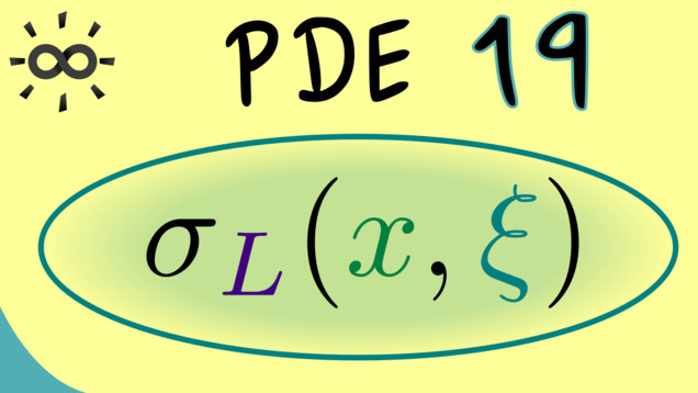
-
Title: Elliptic Differential Operators
-
Series: Partial Differential Equations
-
Chapter: Laplace’s Equation
-
YouTube-Title: Partial Differential Equations 19 | Elliptic Differential Operators
-
Bright video: Watch on YouTube
-
Dark video: Watch on YouTube
-
Ad-free video: Watch Vimeo video
-
Forum: Ask a question in Mattermost
-
Dark-PDF: Download PDF version of the dark video
-
Print-PDF: Download printable PDF version
-
Exercise Download PDF sheets
-
Thumbnail (bright): Download PNG
-
Thumbnail (dark): Download PNG
-
Subtitle on GitHub: pde19_sub_eng.srt
-
Download bright video: Link on Vimeo
-
Download dark video: Link on Vimeo
-
Related videos:
-
Timestamps (n/a)
-
Subtitle in English
1 00:00:00,140 –> 00:00:03,800 Hello and welcome back to Partial Differential Equations,
2 00:00:04,220 –> 00:00:05,980 the video series where we talk a lot
3 00:00:05,980 –> 00:00:08,520 about Laplace’s and Poisson’s equation.
4 00:00:09,220 –> 00:00:11,520 And with todays part 19 I want to
5 00:00:11,520 –> 00:00:14,460 close the topic of Laplace’s equation, because I
6 00:00:14,460 –> 00:00:16,620 also want to talk about other partial differential
7 00:00:16,620 –> 00:00:17,240 equations.
8 00:00:18,000 –> 00:00:20,400 And as you might already know, Laplace’s equation
9 00:00:20,400 –> 00:00:22,880 is a typical example of a so called
10 00:00:22,880 –> 00:00:24,060 elliptic PDE.
11 00:00:24,680 –> 00:00:26,540 Therefore today I want to tell you where
12 00:00:26,540 –> 00:00:29,380 this name comes from and which other kinds
13 00:00:29,380 –> 00:00:30,560 of PDEs we have.
14 00:00:31,320 –> 00:00:33,580 However as always before we start, I first
15 00:00:33,580 –> 00:00:35,340 want to thank all the nice people who
16 00:00:35,340 –> 00:00:37,400 support this channel on Steady, here on Youtube
17 00:00:37,400 –> 00:00:38,660 or via other means.
18 00:00:39,280 –> 00:00:40,900 And please just click the link in the
19 00:00:40,900 –> 00:00:43,320 description and use your Steady account to download
20 00:00:43,320 –> 00:00:45,460 the additional material for all the videos.
21 00:00:46,380 –> 00:00:48,840 And then without further ado, let’s immediately consider
22 00:00:48,840 –> 00:00:52,380 Laplace’s equation, which is given as delta u
23 00:00:52,380 –> 00:00:53,840 is equal to zero.
24 00:00:53,840 –> 00:00:56,700 And if someone asks you about an example
25 00:00:56,700 –> 00:00:59,260 of an elliptic PDE, you can always give
26 00:00:59,260 –> 00:01:00,680 this Laplace’s equation.
27 00:01:01,520 –> 00:01:04,760 Indeed the simplest example would be Laplace’s equation
28 00:01:04,760 –> 00:01:05,900 in two dimensions.
29 00:01:06,880 –> 00:01:09,260 Simply because the one dimensional case would not
30 00:01:09,260 –> 00:01:11,540 define a partial differential equation.
31 00:01:12,100 –> 00:01:14,020 But already in two dimensions we can talk
32 00:01:14,020 –> 00:01:17,540 about partial derivatives with respect to two different
33 00:01:17,540 –> 00:01:19,240 variables x and y.
34 00:01:20,040 –> 00:01:22,120 And in that case we can definitely answer
35 00:01:22,120 –> 00:01:26,160 the question, why we call Laplace’s equation elliptic.
36 00:01:26,780 –> 00:01:29,140 Moreover we can even generalise that to a
37 00:01:29,140 –> 00:01:32,300 linear PDE of order two, where the coefficients
38 00:01:32,300 –> 00:01:35,020 in front of the partial derivatives are constant.
39 00:01:35,740 –> 00:01:38,180 This means the highest derivatives are the same
40 00:01:38,180 –> 00:01:40,700 as in the Laplacian, but we can also
41 00:01:40,700 –> 00:01:42,400 have first order derivatives.
42 00:01:43,280 –> 00:01:45,700 So let’s write down the pure second order
43 00:01:45,700 –> 00:01:48,440 partial derivatives and the first order partial derivatives
44 00:01:48,440 –> 00:01:49,020 here.
45 00:01:49,560 –> 00:01:51,280 And then you know we also have the
46 00:01:51,280 –> 00:01:52,760 mixed second order one.
47 00:01:53,540 –> 00:01:55,660 And if we assume that we only consider
48 00:01:55,660 –> 00:01:58,760 C2 functions u, then the order of the
49 00:01:58,760 –> 00:02:00,660 partial derivatives here does not matter.
50 00:02:01,380 –> 00:02:03,320 And then finally we can also take the
51 00:02:03,320 –> 00:02:06,440 zeroth order, which is just the function u
52 00:02:06,440 –> 00:02:06,940 itself.
53 00:02:07,639 –> 00:02:09,360 And moreover since we want to have a
54 00:02:09,360 –> 00:02:11,880 linear PDE, this means that we can only
55 00:02:11,880 –> 00:02:14,700 connect these parts by the addition, but we
56 00:02:14,700 –> 00:02:17,460 can also scale the different parts as well.
57 00:02:17,660 –> 00:02:19,920 But as already mentioned in the title, these
58 00:02:19,920 –> 00:02:22,160 coefficients should just be constants.
59 00:02:23,200 –> 00:02:25,420 So we just have real numbers a, b,
60 00:02:25,520 –> 00:02:26,540 c and so on.
61 00:02:27,260 –> 00:02:29,160 And now to make the formulas later a
62 00:02:29,160 –> 00:02:31,600 little bit simpler, we can introduce a factor
63 00:02:31,600 –> 00:02:33,560 two in the mixed term here.
64 00:02:34,280 –> 00:02:35,100 And that’s already it.
65 00:02:35,220 –> 00:02:37,140 These are just real numbers.
66 00:02:37,980 –> 00:02:39,780 And moreover the right hand side of this
67 00:02:39,780 –> 00:02:42,400 equation is either given by zero or by
68 00:02:42,400 –> 00:02:42,840 a function.
69 00:02:42,840 –> 00:02:45,940 So we have the homogeneous linear PDE or
70 00:02:45,940 –> 00:02:47,160 the inhomogeneous one.
71 00:02:47,800 –> 00:02:49,320 So in general we can just write a
72 00:02:49,320 –> 00:02:51,280 function g on the right hand side.
73 00:02:52,100 –> 00:02:54,000 Okay, so this is the general form, but
74 00:02:54,000 –> 00:02:56,380 we can already start with simplifications.
75 00:02:56,880 –> 00:02:59,480 For example we could say that the highest
76 00:02:59,480 –> 00:03:02,360 order contributes the most to the PDE.
77 00:03:02,780 –> 00:03:05,020 Therefore we just want to analyse this first
78 00:03:05,020 –> 00:03:08,060 part here, which is already really close to
79 00:03:08,060 –> 00:03:09,140 the Laplacian anyway.
80 00:03:09,740 –> 00:03:12,460 In fact we can easily translate this part
81 00:03:12,460 –> 00:03:15,080 into a nice form by using the Napla
82 00:03:15,080 –> 00:03:15,520 operator.
83 00:03:16,240 –> 00:03:18,620 This is just a differential operator, where the
84 00:03:18,620 –> 00:03:21,280 first component is given by the partial derivative
85 00:03:21,280 –> 00:03:24,380 with respect to x, and the second component
86 00:03:24,380 –> 00:03:27,240 is the partial derivative with respect to y.
87 00:03:27,880 –> 00:03:29,640 And there you might already see, in order
88 00:03:29,640 –> 00:03:32,300 to get the second order out, we have
89 00:03:32,300 –> 00:03:35,260 to use this Napla in the standard inner
90 00:03:35,260 –> 00:03:36,280 product twice.
91 00:03:37,000 –> 00:03:39,940 However since we also need the coefficients, let’s
92 00:03:39,940 –> 00:03:42,500 put them into a 2 times 2 matrix
93 00:03:42,500 –> 00:03:42,800 M.
94 00:03:43,540 –> 00:03:45,340 And this is quite simple, we just have
95 00:03:45,340 –> 00:03:48,760 A B on the diagonal and C off
96 00:03:48,760 –> 00:03:49,280 diagonal.
97 00:03:50,100 –> 00:03:51,980 And there you see it’s a symmetric matrix
98 00:03:51,980 –> 00:03:55,080 with real entries, so a real self-adjoint
99 00:03:55,080 –> 00:03:55,600 matrix.
100 00:03:56,200 –> 00:03:58,580 And now by using this self-adjoint matrix,
101 00:03:58,840 –> 00:04:02,280 we can rewrite these highest order terms of
102 00:04:02,280 –> 00:04:02,980 our PDE.
103 00:04:03,700 –> 00:04:06,080 So we take the standard inner product in
104 00:04:06,080 –> 00:04:06,920 a formal way.
105 00:04:07,520 –> 00:04:09,800 On the right we just have M times
106 00:04:09,800 –> 00:04:12,400 the Napla operator, and on the left we
107 00:04:12,400 –> 00:04:13,740 just have the Napla operator.
108 00:04:14,640 –> 00:04:17,060 And then formally we combine them in the
109 00:04:17,060 –> 00:04:18,899 standard inner product of R2.
110 00:04:19,800 –> 00:04:22,460 So by doing this matrix vector multiplication, and
111 00:04:22,460 –> 00:04:25,320 then the inner product multiplication, you see we
112 00:04:25,320 –> 00:04:28,100 also get this factor 2 in the mixed
113 00:04:28,100 –> 00:04:28,440 term.
114 00:04:29,100 –> 00:04:30,600 So you might see that as a fancy
115 00:04:30,600 –> 00:04:33,680 way of writing our PDE, but it helps
116 00:04:33,680 –> 00:04:36,240 us, because we know a lot about self
117 00:04:36,240 –> 00:04:36,900 -adjoint matrices.
118 00:04:37,900 –> 00:04:40,180 Indeed from linear algebra we know, that we
119 00:04:40,180 –> 00:04:43,340 can always diagonalize a self-adjoint matrix.
120 00:04:44,040 –> 00:04:47,920 More precisely so-called normal matrices are exactly
121 00:04:47,920 –> 00:04:51,600 the ones that are unitarily diagonalisable, and self
122 00:04:51,600 –> 00:04:53,260 -adjoint matrices are normal.
123 00:04:54,120 –> 00:04:56,540 Moreover since we only deal with real numbers
124 00:04:56,540 –> 00:04:59,420 here, and self-adjoint matrices only have real
125 00:04:59,420 –> 00:05:02,760 eigenvalues, we don’t need the complex numbers for
126 00:05:02,760 –> 00:05:04,320 the diagonalisation at all.
127 00:05:04,820 –> 00:05:07,520 In other words the unitary matrix capital U
128 00:05:07,520 –> 00:05:09,960 is actually an orthogonal matrix.
129 00:05:10,820 –> 00:05:13,720 And by definition this simply means that UT U
130 00:05:13,720 –> 00:05:16,760 is equal to the identity matrix.
131 00:05:17,500 –> 00:05:18,980 And now what we can do is to
132 00:05:18,980 –> 00:05:23,320 form UT M U, and we get out a diagonal
133 00:05:23,320 –> 00:05:23,860 matrix.
134 00:05:24,260 –> 00:05:26,540 And you might also know from linear algebra,
135 00:05:26,540 –> 00:05:29,920 that we find the eigenvalues of M on
136 00:05:29,920 –> 00:05:30,500 the diagonal.
137 00:05:31,420 –> 00:05:33,040 And in order to keep it simple, let’s
138 00:05:33,040 –> 00:05:36,000 call this diagonal matrix just capital D.
139 00:05:36,960 –> 00:05:39,100 Obviously you can see U as a change
140 00:05:39,100 –> 00:05:43,360 of values transformation, that transforms our coordinates in
141 00:05:43,360 –> 00:05:45,800 such a way, that M acts as a
142 00:05:45,800 –> 00:05:47,200 diagonal matrix in the end.
143 00:05:47,900 –> 00:05:49,620 And this is exactly what we want to
144 00:05:49,620 –> 00:05:53,820 simplify this quadratic form, that describes our PDE.
145 00:05:54,380 –> 00:05:56,700 So maybe more concretely you could say, we
146 00:05:56,700 –> 00:06:00,060 have the two coordinates alpha and beta, and
147 00:06:00,060 –> 00:06:02,480 now we use them instead of the nabla
148 00:06:02,480 –> 00:06:03,360 operator above.
149 00:06:04,320 –> 00:06:06,180 And now you see we can just substitute
150 00:06:06,180 –> 00:06:09,700 our M with U D Ut.
151 00:06:10,460 –> 00:06:12,320 And by doing that we actually see the
152 00:06:12,320 –> 00:06:15,680 change of variables here by Ut alpha beta.
153 00:06:16,380 –> 00:06:18,780 So let’s denote the new variables alpha and
154 00:06:18,780 –> 00:06:20,420 beta with a tilde on top.
155 00:06:20,420 –> 00:06:23,680 Hence by using these new variables, we just
156 00:06:23,680 –> 00:06:26,560 have a diagonal matrix inside the inner product.
157 00:06:27,280 –> 00:06:29,940 So suddenly this whole quadratic form here is
158 00:06:29,940 –> 00:06:30,720 quite simple.
159 00:06:31,380 –> 00:06:35,080 It’s just lambda one times alpha squared plus
160 00:06:35,080 –> 00:06:37,400 lambda two times beta squared.
161 00:06:38,100 –> 00:06:38,520 And that’s it.
162 00:06:38,620 –> 00:06:40,720 This is the simple form of our quadratic
163 00:06:40,720 –> 00:06:44,560 form, that describes the parts of highest order
164 00:06:44,560 –> 00:06:45,560 in our PDE.
165 00:06:46,380 –> 00:06:49,120 And depending on the eigenvalues lambda one and
166 00:06:49,120 –> 00:06:52,540 lambda two, we immediately see different cases in
167 00:06:52,540 –> 00:06:53,020 this formula.
168 00:06:53,820 –> 00:06:56,020 In fact it’s all about the product lambda
169 00:06:56,020 –> 00:06:58,360 one times lambda two, which is just the
170 00:06:58,360 –> 00:06:59,680 determinant of M.
171 00:07:00,340 –> 00:07:02,160 So let’s look at the first case, where
172 00:07:02,160 –> 00:07:04,520 this product is actually positive.
173 00:07:05,400 –> 00:07:08,840 Hence either both eigenvalues are positive, or both
174 00:07:08,840 –> 00:07:10,300 eigenvalues are negative.
175 00:07:11,100 –> 00:07:13,240 And in both cases we can simply look
176 00:07:13,240 –> 00:07:16,340 at the contour lines of our quadratic form
177 00:07:16,340 –> 00:07:16,800 here.
178 00:07:17,520 –> 00:07:19,680 So the x-axis here is alpha tilde,
179 00:07:19,880 –> 00:07:22,020 and the y-axis is beta tilde.
180 00:07:22,800 –> 00:07:24,260 And there you should know, that a contour
181 00:07:24,260 –> 00:07:26,660 line is just the pre-image of a
182 00:07:26,660 –> 00:07:27,000 constant.
183 00:07:27,760 –> 00:07:29,740 So the outcome here should be equal to
184 00:07:29,740 –> 00:07:32,420 a constant, and now you might recognise, that
185 00:07:32,420 –> 00:07:34,740 this looks similar to the equation of a
186 00:07:34,740 –> 00:07:35,040 circle.
187 00:07:35,860 –> 00:07:38,140 And actually by using coefficients lambda one and
188 00:07:38,140 –> 00:07:40,660 lambda two, you squeeze the circle, so what
189 00:07:40,660 –> 00:07:43,320 we get is the formula for an ellipse.
190 00:07:43,880 –> 00:07:46,120 Depending on the constant on the right it’s
191 00:07:46,120 –> 00:07:48,720 bigger or smaller, but it always is an
192 00:07:48,720 –> 00:07:49,080 ellipse.
193 00:07:49,880 –> 00:07:52,080 So in that case here contour lines are
194 00:07:52,080 –> 00:07:53,980 always given by ellipses.
195 00:07:54,660 –> 00:07:57,000 And because of that we call the corresponding
196 00:07:57,000 –> 00:07:58,980 PDE elliptic.
197 00:07:59,900 –> 00:08:01,720 And you know in the case of Laplace’s
198 00:08:01,720 –> 00:08:04,680 equation, we have lambda one and lambda two
199 00:08:04,680 –> 00:08:05,760 given as one.
200 00:08:06,420 –> 00:08:09,000 There we don’t even need to diagonalize, because
201 00:08:09,000 –> 00:08:11,900 M already has ones on the diagonal anyway.
202 00:08:12,420 –> 00:08:14,280 But now you know that we also get
203 00:08:14,280 –> 00:08:17,380 an elliptic PDE, if we stretch with some
204 00:08:17,380 –> 00:08:17,900 factors.
205 00:08:18,640 –> 00:08:21,300 However we get a different case, if the
206 00:08:21,300 –> 00:08:23,820 signs of lambda one and lambda two are
207 00:08:23,820 –> 00:08:24,620 not the same.
208 00:08:25,380 –> 00:08:27,580 So in this case the product is definitely
209 00:08:27,580 –> 00:08:28,160 negative.
210 00:08:29,080 –> 00:08:30,960 So by looking at the contour line, we
211 00:08:30,960 –> 00:08:33,140 could say that in front of beta squared
212 00:08:33,140 –> 00:08:34,780 we have a minus sign.
213 00:08:35,380 –> 00:08:37,240 And then we definitely don’t get an ellipse,
214 00:08:37,480 –> 00:08:39,580 we get a so-called hyperbola.
215 00:08:39,580 –> 00:08:42,580 So you see just by changing one sign,
216 00:08:42,740 –> 00:08:45,500 the behaviour of our quadratic form here is
217 00:08:45,500 –> 00:08:46,520 completely different.
218 00:08:47,180 –> 00:08:49,560 So for example this contour line here is
219 00:08:49,560 –> 00:08:51,560 not bounded in the plane anymore.
220 00:08:52,320 –> 00:08:54,760 And in fact this behaviour translates to the
221 00:08:54,760 –> 00:08:58,200 corresponding PDE, and we speak of a hyperbolic
222 00:08:58,200 –> 00:08:58,660 PDE.
223 00:08:59,460 –> 00:09:01,680 And just by looking at the corresponding matrix
224 00:09:01,680 –> 00:09:04,540 M, we can immediately give an example of
225 00:09:04,540 –> 00:09:05,300 such a PDE.
226 00:09:05,300 –> 00:09:08,020 We just take plus one for the derivative
227 00:09:08,020 –> 00:09:11,340 with respect to x, and minus one for
228 00:09:11,340 –> 00:09:13,580 the derivative with respect to y.
229 00:09:14,240 –> 00:09:16,200 So it also looks quite simple, but the
230 00:09:16,200 –> 00:09:19,760 behaviour of the solutions is completely different compared
231 00:09:19,760 –> 00:09:22,080 to the solutions of Laplace’s equation.
232 00:09:22,820 –> 00:09:25,080 Indeed this is something we will discuss in
233 00:09:25,080 –> 00:09:26,860 later videos of this series.
234 00:09:27,580 –> 00:09:29,940 However first we will actually talk about the
235 00:09:29,940 –> 00:09:33,000 next case, where the product is exactly equal
236 00:09:33,000 –> 00:09:33,520 to zero.
237 00:09:33,520 –> 00:09:36,220 Which simply tells us that one of the
238 00:09:36,220 –> 00:09:38,220 two eigenvalues has to vanish.
239 00:09:38,920 –> 00:09:41,860 Hence in that case one variable does not
240 00:09:41,860 –> 00:09:43,460 have a second order term.
241 00:09:43,980 –> 00:09:45,700 And i can immediately give you an example
242 00:09:45,700 –> 00:09:46,220 of that.
243 00:09:46,560 –> 00:09:49,240 Here we have the second order partial derivative
244 00:09:49,240 –> 00:09:51,760 with respect to x, but then on the
245 00:09:51,760 –> 00:09:54,260 right we only have the first order with
246 00:09:54,260 –> 00:09:55,280 respect to y.
247 00:09:55,940 –> 00:09:57,480 So you see if we want to sketch
248 00:09:57,480 –> 00:10:00,720 that with contour lines, we also have to
249 00:10:00,720 –> 00:10:03,180 consider the first order parts as well.
250 00:10:03,520 –> 00:10:06,000 And with this example in mind it should
251 00:10:06,000 –> 00:10:08,140 be immediately clear that we get a parabola
252 00:10:08,140 –> 00:10:08,520 out.
253 00:10:09,260 –> 00:10:11,580 And therefore in this case we speak of
254 00:10:11,580 –> 00:10:12,920 parabolic PDEs.
255 00:10:13,600 –> 00:10:15,660 And indeed in the next video I want
256 00:10:15,660 –> 00:10:18,180 to discuss the typical example of such a
257 00:10:18,180 –> 00:10:19,240 parabolic PDE.
258 00:10:19,860 –> 00:10:21,920 However for that we also need the general
259 00:10:21,920 –> 00:10:25,280 definition, where we don’t restrict ourselves to two
260 00:10:25,280 –> 00:10:25,740 dimensions.
261 00:10:26,560 –> 00:10:28,440 And in addition to that we can also
262 00:10:28,440 –> 00:10:31,080 look at higher orders for the partial derivatives.
263 00:10:31,080 –> 00:10:33,260 And in order to do that let’s put
264 00:10:33,260 –> 00:10:36,040 the PDE in a so-called differential operator.
265 00:10:36,680 –> 00:10:38,680 And it will be a linear differential operator,
266 00:10:38,860 –> 00:10:40,480 so I just call it capital L.
267 00:10:41,140 –> 00:10:43,020 And the definition is more or less the
268 00:10:43,020 –> 00:10:44,040 same as before.
269 00:10:44,300 –> 00:10:47,480 We have partial derivatives and they only occur
270 00:10:47,480 –> 00:10:48,560 in a linear sense.
271 00:10:49,180 –> 00:10:51,760 So the function u we consider here is
272 00:10:51,760 –> 00:10:53,460 defined on Rn.
273 00:10:54,260 –> 00:10:56,400 So we have n variables, but the highest
274 00:10:56,400 –> 00:10:59,300 order of our PDE should be given by
275 00:10:59,300 –> 00:11:00,380 the variable m.
276 00:11:01,080 –> 00:11:03,080 And then we just go through all possible
277 00:11:03,080 –> 00:11:06,120 multi indices alpha, where we have the partial
278 00:11:06,120 –> 00:11:08,820 derivatives here and the coefficients there.
279 00:11:09,500 –> 00:11:11,460 So you see in general it’s allowed that
280 00:11:11,460 –> 00:11:14,240 the coefficients depend on the variable x.
281 00:11:14,880 –> 00:11:16,200 And then we can do a similar thing
282 00:11:16,200 –> 00:11:18,480 to before, when we just look at the
283 00:11:18,480 –> 00:11:19,820 highest possible orders.
284 00:11:20,080 –> 00:11:21,460 And what we get out is what we
285 00:11:21,460 –> 00:11:22,840 call the principal symbol.
286 00:11:23,520 –> 00:11:25,840 And the general idea of a symbol of
287 00:11:25,840 –> 00:11:28,560 a differential operator is that we replace the
288 00:11:28,560 –> 00:11:30,140 derivatives with variables.
289 00:11:31,080 –> 00:11:32,860 And then the common name is a lowercase
290 00:11:32,860 –> 00:11:34,700 sigma with index L.
291 00:11:35,320 –> 00:11:36,680 And it’s a function with a lot of
292 00:11:36,680 –> 00:11:37,160 variables.
293 00:11:37,440 –> 00:11:39,300 And the first ones are given by x
294 00:11:39,300 –> 00:11:41,000 and the other ones by xc.
295 00:11:41,740 –> 00:11:43,660 And now in the definition we only take
296 00:11:43,660 –> 00:11:46,440 the highest order, which is given by m.
297 00:11:46,900 –> 00:11:49,040 And then we have the coefficients and the
298 00:11:49,040 –> 00:11:52,120 derivatives are replaced by our variables xc.
299 00:11:52,760 –> 00:11:55,200 And then they get the power alpha, which
300 00:11:55,200 –> 00:11:58,500 means xc1 gets alpha 1, xc2 alpha 2
301 00:11:58,500 –> 00:11:59,080 and so on.
302 00:11:59,080 –> 00:12:01,600 And then in the end everything is multiplied,
303 00:12:02,220 –> 00:12:04,740 which is common in this multi index notation.
304 00:12:05,540 –> 00:12:07,640 Hence if we fix the point x in
305 00:12:07,640 –> 00:12:10,640 the principal symbol we actually get a polynomial
306 00:12:10,640 –> 00:12:11,520 in xi.
307 00:12:12,180 –> 00:12:14,280 So for example before we just had a
308 00:12:14,280 –> 00:12:16,700 quadratic polynomial in these variables.
309 00:12:17,480 –> 00:12:19,960 And then the elliptic case was given when
310 00:12:19,960 –> 00:12:22,800 all coefficients in front had the same sign.
311 00:12:23,320 –> 00:12:25,500 And now we can also define that for
312 00:12:25,500 –> 00:12:29,000 a general differential operator L and the PDE
313 00:12:29,000 –> 00:12:31,040 Lu is equal to 0.
314 00:12:31,640 –> 00:12:34,920 Both things will carry the name elliptic if
315 00:12:34,920 –> 00:12:37,840 our principal symbol does not vanish.
316 00:12:38,520 –> 00:12:41,120 So regardless of which c we put in
317 00:12:41,120 –> 00:12:42,860 we never get out 0.
318 00:12:43,580 –> 00:12:45,580 Of course the only exception has to be
319 00:12:45,580 –> 00:12:48,240 the point 0 as well, because there the
320 00:12:48,240 –> 00:12:49,540 polynomial will vanish.
321 00:12:50,240 –> 00:12:52,440 Otherwise you should see this is a straightforward
322 00:12:52,440 –> 00:12:55,680 generalisation of our property from the quadratic polynomial
323 00:12:55,680 –> 00:12:56,200 before.
324 00:12:56,200 –> 00:12:59,880 However since here our coefficients depend on x,
325 00:13:00,060 –> 00:13:02,980 we want to have this property independent of
326 00:13:02,980 –> 00:13:03,840 the chosen x.
327 00:13:04,500 –> 00:13:06,400 And usually as you know x goes through
328 00:13:06,400 –> 00:13:08,000 a domain that we call omega.
329 00:13:08,780 –> 00:13:10,620 So there we have the general definition and
330 00:13:10,620 –> 00:13:12,720 we can immediately check it for an example.
331 00:13:13,560 –> 00:13:15,360 And obviously first we should check it for
332 00:13:15,360 –> 00:13:17,440 the Laplacian on Rn.
333 00:13:18,280 –> 00:13:21,160 Obviously this one should also be elliptic by
334 00:13:21,160 –> 00:13:22,520 using the definition above.
335 00:13:23,050 –> 00:13:25,280 And this is quite simple because our principal
336 00:13:25,280 –> 00:13:28,400 symbol is just given by a quadratic polynomial
337 00:13:28,400 –> 00:13:29,000 again.
338 00:13:29,560 –> 00:13:32,660 Indeed the second order partial derivatives just give
339 00:13:32,660 –> 00:13:37,040 us xc1 squared plus xc2 squared until we
340 00:13:37,040 –> 00:13:38,820 reach xcn squared.
341 00:13:39,540 –> 00:13:42,480 And obviously this can only vanish if all
342 00:13:42,480 –> 00:13:44,240 xc’s are equal to 0.
343 00:13:45,080 –> 00:13:47,200 And moreover you also see that we don’t
344 00:13:47,200 –> 00:13:50,620 change the elliptic property if we scale some
345 00:13:50,620 –> 00:13:53,040 of our variables by a positive constant.
346 00:13:53,880 –> 00:13:55,820 Therefore you can already give a lot of
347 00:13:55,820 –> 00:13:58,400 different elliptic properties on Rn.
348 00:13:59,180 –> 00:14:01,220 However now let’s say we have an elliptic
349 00:14:01,220 –> 00:14:04,020 operator on Rn, but now we add an
350 00:14:04,020 –> 00:14:06,180 additional dimension t to it.
351 00:14:06,900 –> 00:14:09,880 This means we consider functions u with n
352 00:14:09,880 –> 00:14:11,240 plus 1 variables.
353 00:14:11,940 –> 00:14:14,300 And only with respect to the first n
354 00:14:14,300 –> 00:14:16,800 variables I want to have an elliptic operator.
355 00:14:17,360 –> 00:14:19,780 And again the typical example would be just
356 00:14:19,780 –> 00:14:21,880 the Laplacian in n variables.
357 00:14:22,800 –> 00:14:25,120 But now the function u also has a
358 00:14:25,120 –> 00:14:28,100 well-defined derivative with respect to t.
359 00:14:28,660 –> 00:14:31,520 This means we can actually combine this derivative
360 00:14:31,520 –> 00:14:33,580 with our elliptic operator L.
361 00:14:34,300 –> 00:14:36,400 This means here on the right hand side
362 00:14:36,400 –> 00:14:38,820 L does not care about the variable t
363 00:14:38,820 –> 00:14:39,420 at all.
364 00:14:40,100 –> 00:14:41,920 And now this combination where we have an
365 00:14:41,920 –> 00:14:44,760 elliptic operator on the right hand side and
366 00:14:44,760 –> 00:14:47,160 a first order derivative on the left is
367 00:14:47,160 –> 00:14:48,820 called a parabolic operator.
368 00:14:49,680 –> 00:14:51,860 Which means now we also have the general
369 00:14:51,860 –> 00:14:54,200 definition of a parabolic PDE.
370 00:14:54,820 –> 00:14:56,940 And you also immediately see that this definition
371 00:14:56,940 –> 00:14:59,760 is consistent with the two-dimensional case from
372 00:14:59,760 –> 00:15:00,040 above.
373 00:15:00,660 –> 00:15:02,720 And moreover, as you might already know, the
374 00:15:02,720 –> 00:15:05,280 typical example is that we choose L as
375 00:15:05,280 –> 00:15:07,800 the Laplacian and then we get the so
376 00:15:07,800 –> 00:15:09,020 -called heat equation.
377 00:15:09,580 –> 00:15:12,160 So you can already remember the heat equation
378 00:15:12,160 –> 00:15:14,660 is a so-called parabolic PDE.
379 00:15:15,420 –> 00:15:17,300 And this is already the cliffhanger for the
380 00:15:17,300 –> 00:15:20,160 next video, because there we will start talking
381 00:15:20,160 –> 00:15:21,460 about this heat equation.
382 00:15:22,200 –> 00:15:23,360 So I really hope I meet you there
383 00:15:23,360 –> 00:15:25,240 again and I wish you a nice day.
384 00:15:25,520 –> 00:15:25,940 Bye, bye.
-
Quiz Content (n/a)
-
Date of video: 2026-07-24
-
Last update: 2026-07

