-
Title: QR decomposition (for square matrices)
-
YouTube-Title: QR decomposition (for square matrices)
-
Bright video: Watch on YouTube
-
Dark video: Watch on YouTube
-
Ad-free video: Watch Vimeo video
-
Forum: Ask a question in Mattermost
-
Dark-PDF: Download PDF version of the dark video
-
Print-PDF: Download printable PDF version
-
Thumbnail (bright): Download PNG
-
Thumbnail (dark): Download PNG
-
Subtitle on GitHub: qr-deco01_sub_eng.srt
-
Download bright video: Link on Vimeo
-
Download dark video: Link on Vimeo
-
Timestamps (n/a)
-
Subtitle in English
1 00:00:00.785 –> 00:00:04.615 Hello and welcome back to new video about Linear Algebra.
2 00:00:05.665 –> 00:00:08.815 First I want to thank all the nice supporters on Steady.
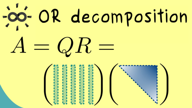
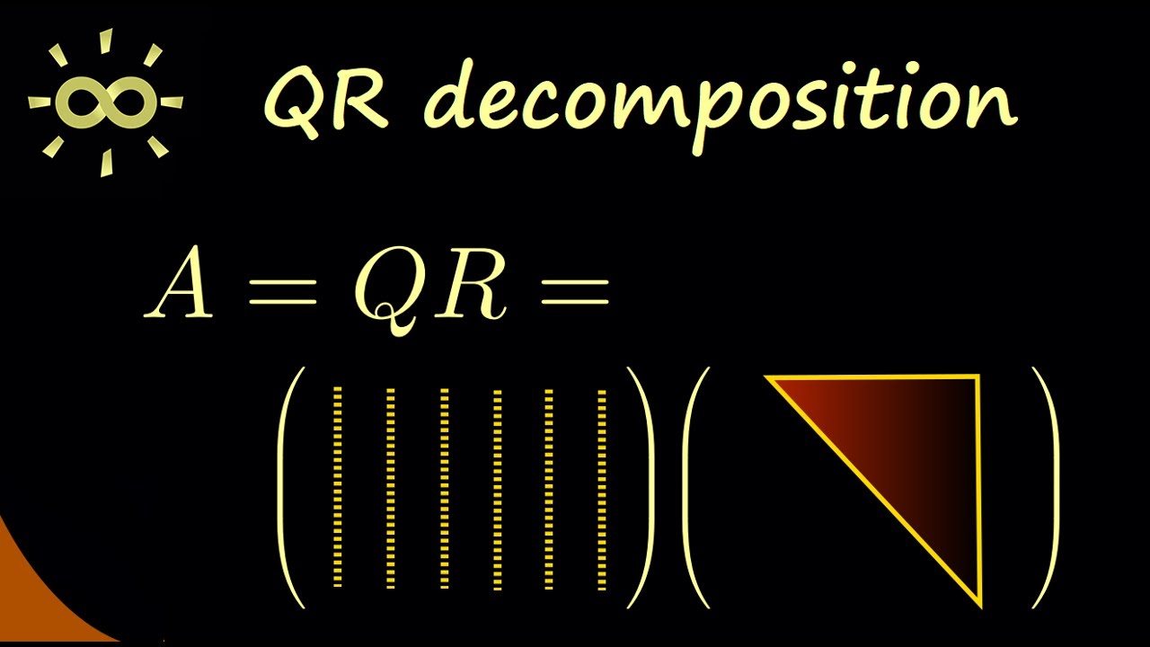
3 00:00:09.845 –> 00:00:14.775 Today’s topic is the QR decomposition for square matrixes.
4 00:00:15.885 –> 00:00:18.775 Here I want to show you it for invertible matrix,
5 00:00:19.155 –> 00:00:21.855 but you will see that the generalization is
6 00:00:21.855 –> 00:00:23.095 not a problem in the end.
7 00:00:24.235 –> 00:00:27.815 For this reason, we choose our matrix A as a square matrix,
8 00:00:28.105 –> 00:00:30.055 which is also invertible.
9 00:00:31.075 –> 00:00:32.655 Now what we want to do is
10 00:00:32.715 –> 00:00:37.135 to decompose our matrix A into the product of two matrices,
11 00:00:37.225 –> 00:00:40.015 which we’ll call Q and R.
12 00:00:40.925 –> 00:00:44.655 Sometimes this whole thing is also called the QU
13 00:00:44.655 –> 00:00:49.575 decomposition because the matrix R on the right should be
14 00:00:49.635 –> 00:00:51.455 an upper triangular matrix.
15 00:00:52.565 –> 00:00:56.615 This means that it looks the same as in the LU decomposition,
16 00:00:57.755 –> 00:01:00.015 so there could be values on the diagonal
17 00:01:00.235 –> 00:01:01.655 and above the diagonal,
18 00:01:02.115 –> 00:01:05.255 but below the diagonal there are only zeros.
19 00:01:07.115 –> 00:01:10.055 And on the other hand we have our matrix Q,
20 00:01:10.345 –> 00:01:13.535 which should be an orthogonal or unitary matrix.
21 00:01:14.595 –> 00:01:17.495 If we deal in the real vector space R^n,
22 00:01:17.675 –> 00:01:21.055 we want here an orthogonal matrix, which means
23 00:01:21.285 –> 00:01:23.095 that the matrix is invertible
24 00:01:23.595 –> 00:01:28.055 and that the transpose is the same as the inverse of Q.
25 00:01:29.795 –> 00:01:32.575 And if we deal in the complex vector space C^n,
26 00:01:32.635 –> 00:01:36.295 we want a unitary matrix, which means roughly the same.
27 00:01:36.635 –> 00:01:38.575 But here we use the adjoint
28 00:01:38.915 –> 00:01:41.975 and it should be the same as the inverse of Q.
29 00:01:43.655 –> 00:01:46.065 However, we can summarize both things.
30 00:01:46.445 –> 00:01:50.985 If we say that the columns of Q form an orthonormal basis,
31 00:01:52.245 –> 00:01:56.385 and indeed that’s the essential part of the QR decomposition,
32 00:01:57.245 –> 00:02:00.905 we make an ONB and write it into the columns of Q
33 00:02:01.365 –> 00:02:06.065 and also generate an easy upper triangular matrix R, such
34 00:02:06.065 –> 00:02:09.465 that the product of both gives us our matrix A back.
35 00:02:10.725 –> 00:02:13.785 So now please recall an orthonormal basis
36 00:02:14.165 –> 00:02:15.305 or in short, an ONB,
37 00:02:15.305 –> 00:02:19.185 is a basis where each element has length one
38 00:02:19.685 –> 00:02:22.105 and two different elements are orthogonal.
39 00:02:23.475 –> 00:02:24.945 Hence, it shouldn’t surprise you
40 00:02:25.055 –> 00:02:28.545 that the whole QR decomposition is related to another thing,
41 00:02:28.595 –> 00:02:31.185 which is called the Gram-Schmidt process.
42 00:02:33.485 –> 00:02:36.505 In fact, I would say they are completely the same thing.
43 00:02:38.055 –> 00:02:40.625 Okay, then let’s start with the calculation.
44 00:02:42.675 –> 00:02:45.465 A square matrix has exactly as many rows as columns,
45 00:02:45.685 –> 00:02:47.305 and maybe to keep it well arranged,
46 00:02:47.595 –> 00:02:49.665 let’s look at three columns.
47 00:02:50.645 –> 00:02:53.545 So let’s call our columns a one, a two, a three,
48 00:02:53.915 –> 00:02:57.425 which means each vector here has three components.
49 00:02:58.995 –> 00:03:00.405 What we now want to do is
50 00:03:00.405 –> 00:03:03.845 to transform these three vectors into an ONB.
51 00:03:05.095 –> 00:03:08.685 Hence, what we get out is our matrix Q, also
52 00:03:08.685 –> 00:03:13.245 with three columns, which we call q1, q2, and q3.
53 00:03:14.035 –> 00:03:18.605 Because all these columns should have length one, we start
54 00:03:18.705 –> 00:03:21.205 by normalizing the first vector here.
55 00:03:22.805 –> 00:03:25.335 This gives us now the definition for q1,
56 00:03:25.625 –> 00:03:29.775 which should be our vector, a one divided by the length
57 00:03:29.775 –> 00:03:32.055 of the vector, so the norm of a one.
58 00:03:33.565 –> 00:03:36.705 So you see calculating q1 is always easy,
59 00:03:37.165 –> 00:03:39.745 but for q2 we have to do a little bit more.
60 00:03:40.975 –> 00:03:44.425 Here you see the picture, this is the direction of q1,
61 00:03:44.885 –> 00:03:46.545 and this one is a two.
62 00:03:47.005 –> 00:03:49.625 And you see by just normalizing a two,
63 00:03:50.005 –> 00:03:52.185 you don’t get an orthogonal vector.
64 00:03:53.935 –> 00:03:55.385 This means that what we have
65 00:03:55.625 –> 00:03:58.785 to do is calculating an orthogonal projection.
66 00:04:00.565 –> 00:04:02.055 Then the picture looks like this
67 00:04:02.315 –> 00:04:04.415 and it’s just a vector decomposition.
68 00:04:04.875 –> 00:04:07.815 And the blue vector we can calculate with the help
69 00:04:07.835 –> 00:04:10.375 of the inner product here.
70 00:04:10.405 –> 00:04:12.575 This just denotes the standard inner product
71 00:04:12.715 –> 00:04:15.215 or sometimes also called scalar product.
72 00:04:15.715 –> 00:04:18.615 And if you calculate it, you get the length
73 00:04:18.715 –> 00:04:20.015 of this vector here.
74 00:04:20.805 –> 00:04:24.055 Then by multiplying of the normalized vector q1,
75 00:04:24.235 –> 00:04:25.935 you also get the direction in
76 00:04:26.075 –> 00:04:28.015 and you get out this arrow here.
77 00:04:28.725 –> 00:04:30.415 However, this is not what we want.
78 00:04:30.555 –> 00:04:33.815 We want the orange arrow here, so let’s call it
79 00:04:34.415 –> 00:04:39.045 a two perpendicular and how to calculate that.
80 00:04:39.185 –> 00:04:40.525 You should see immediately
81 00:04:40.525 –> 00:04:42.485 because you can write down the vector
82 00:04:42.785 –> 00:04:46.005 and then you see this is just a vector subtraction.
83 00:04:46.505 –> 00:04:50.925 So if you write a two minus the blue vector here,
84 00:04:51.675 –> 00:04:56.455 and this gives thedo orange vector, you see it’s orthogonal
85 00:04:56.995 –> 00:04:59.415 to q1, but not yet normalized.
86 00:05:00.355 –> 00:05:02.495 And this is what we now can simply do as
87 00:05:02.495 –> 00:05:06.375 before we take our vector a two perpendicular
88 00:05:06.835 –> 00:05:08.975 and divide by its length.
89 00:05:11.805 –> 00:05:14.135 Okay? And what we get out is our q2,
90 00:05:14.595 –> 00:05:16.615 and you should always read that as a definition.
91 00:05:16.835 –> 00:05:18.495 So this defines q2
92 00:05:18.955 –> 00:05:22.055 and this one here, defined q1.
93 00:05:23.715 –> 00:05:25.255 Now before doing q3,
94 00:05:25.625 –> 00:05:28.615 let’s first talk about our matrix R as well.
95 00:05:29.715 –> 00:05:31.935 Let us just use the space up here.
96 00:05:34.915 –> 00:05:37.815 Now, please recall what we want for the matrix R.
97 00:05:37.955 –> 00:05:40.655 We want to multiply Q with R such
98 00:05:40.655 –> 00:05:43.695 that we get out our original matrix A.
99 00:05:44.595 –> 00:05:48.255 So for example, if you look at the first column in R,
100 00:05:48.955 –> 00:05:50.335 you have three numbers here,
101 00:05:52.315 –> 00:05:55.535 and the first one gets multiplied by the first column here,
102 00:05:55.875 –> 00:05:57.485 the second one by the second column,
103 00:05:57.545 –> 00:05:59.645 and the third one by the third column here.
104 00:05:59.985 –> 00:06:02.725 So, and this one should get you
105 00:06:03.185 –> 00:06:05.485 to the original column a one.
106 00:06:06.745 –> 00:06:09.245 In other words, we have a linear combination
107 00:06:09.545 –> 00:06:11.045 of these columns here
108 00:06:11.105 –> 00:06:14.605 and what we put in the matrix R are just a coefficient.
109 00:06:15.955 –> 00:06:18.485 Okay? Then let’s fill in the first column here.
110 00:06:18.985 –> 00:06:20.405 So I erase that again,
111 00:06:20.625 –> 00:06:24.245 and now we look how to get to a one by a linear combination
112 00:06:24.585 –> 00:06:25.965 of these vectors here.
113 00:06:26.985 –> 00:06:30.205 Now if you look at this equation here, you can bring
114 00:06:30.205 –> 00:06:31.205 that on the other side,
115 00:06:31.225 –> 00:06:32.845 and then you have the linear combination,
116 00:06:33.015 –> 00:06:37.925 which means this number here, the norm of a one is exactly
117 00:06:38.505 –> 00:06:40.925 the number that you should put in at
118 00:06:40.925 –> 00:06:42.045 the first position here.
119 00:06:44.065 –> 00:06:45.765 And because there’s no q2
120 00:06:45.865 –> 00:06:49.285 or q3 involved here, we get the zeros here
121 00:06:49.465 –> 00:06:51.165 as we wanted from the beginning.
122 00:06:52.305 –> 00:06:55.925 So the idea is here that you don’t calculate again, formulas
123 00:06:55.925 –> 00:06:59.445 for the matrix R, but rather you put in the numbers
124 00:06:59.625 –> 00:07:03.325 you calculate in these steps immediately into the matrix R.
125 00:07:04.595 –> 00:07:07.485 Okay? And now we can look at the second column here as well.
126 00:07:07.855 –> 00:07:10.325 There we look what is the linear combination
127 00:07:10.985 –> 00:07:14.365 for these vectors to get out to a two.
128 00:07:14.915 –> 00:07:16.285 Okay, here you see a two.
129 00:07:16.465 –> 00:07:18.445 So you can put that on the other side.
130 00:07:18.865 –> 00:07:20.045 And there you have q1.
131 00:07:20.425 –> 00:07:24.565 So this part here is exactly the coefficient
132 00:07:24.785 –> 00:07:25.965 in front of q1.
133 00:07:26.465 –> 00:07:29.085 So this should be up here.
134 00:07:31.045 –> 00:07:32.495 It’s the same idea as before.
135 00:07:32.605 –> 00:07:34.015 When calculating this number,
136 00:07:34.315 –> 00:07:37.335 you can store it immediately into the matrix R
137 00:07:38.465 –> 00:07:40.445 and the coefficient in front of q2.
138 00:07:40.545 –> 00:07:42.725 You see here, it’s the same as before.
139 00:07:43.035 –> 00:07:45.125 It’s the norm of this vector here
140 00:07:45.425 –> 00:07:47.725 and you put that on the diagonal.
141 00:07:49.515 –> 00:07:52.765 It’s not the same number as before, but it’s the same idea.
142 00:07:53.025 –> 00:07:55.165 So you get norms on the diagonal
143 00:07:55.465 –> 00:07:58.765 and above the diagonal you will get inner products.
144 00:08:00.075 –> 00:08:03.045 Also, what you see here is no q3 involved, and
145 00:08:03.045 –> 00:08:05.205 therefore here is also a zero.
146 00:08:06.525 –> 00:08:09.535 Okay? And now we are ready to deal with the last step,
147 00:08:09.555 –> 00:08:11.255 the last column in this example.
148 00:08:14.465 –> 00:08:16.285 Now we want to calculate something
149 00:08:16.285 –> 00:08:18.245 that I call a three perpendicular,
150 00:08:18.495 –> 00:08:21.645 which means we calculate orthogonal projections
151 00:08:21.745 –> 00:08:23.485 and subtract them from a three.
152 00:08:25.145 –> 00:08:27.885 So the first part would be calculating the projection
153 00:08:27.985 –> 00:08:32.405 of a three into into q1 direction, which looks the same as
154 00:08:32.405 –> 00:08:34.205 before, uh, this picture.
155 00:08:34.785 –> 00:08:39.205 But then we also have to consider the direction into q2.
156 00:08:39.545 –> 00:08:43.845 So we also calculate this one and subtract it.
157 00:08:47.095 –> 00:08:48.915 If you want to do a picture of this,
158 00:08:49.015 –> 00:08:50.915 it would look a little bit more complicated.
159 00:08:51.135 –> 00:08:52.275 So I tried that here.
160 00:08:52.535 –> 00:08:55.765 So you have a vector, a three, the directions q1
161 00:08:55.825 –> 00:08:58.365 and q2, they form a plane.
162 00:08:59.315 –> 00:09:02.325 However, you have two normal projections as before.
163 00:09:02.505 –> 00:09:04.365 So the one in q1 direction
164 00:09:04.425 –> 00:09:06.445 and the other one in q2 direction.
165 00:09:07.385 –> 00:09:08.725 If you then sum them up,
166 00:09:08.905 –> 00:09:12.445 you get indeed the projection onto the plane
167 00:09:13.865 –> 00:09:17.485 and therefore also the normal part we are interested in.
168 00:09:19.415 –> 00:09:22.585 Okay? And at this point, I think you know what to do.
169 00:09:22.925 –> 00:09:26.705 So this coefficient in front of q1 is of course the thing
170 00:09:26.815 –> 00:09:29.065 that should go into the matrix R
171 00:09:29.525 –> 00:09:34.255 and the upper right corner in the same way,
172 00:09:34.435 –> 00:09:38.575 the part in front of q2 is the coefficient in front of q2.
173 00:09:38.955 –> 00:09:40.855 So it goes into the matrix R.
174 00:09:41.755 –> 00:09:45.215 In this point, The only part
175 00:09:45.215 –> 00:09:48.775 that is now missing is q3, but you know how to calculate it.
176 00:09:49.115 –> 00:09:52.535 We just normalize our a three perpendicular.
177 00:09:53.155 –> 00:09:55.135 So dividing by the norm
178 00:09:57.915 –> 00:10:01.055 and the same way as before, this norm here has
179 00:10:01.055 –> 00:10:02.855 to be on the diagonal of R.
180 00:10:03.235 –> 00:10:05.015 So here in this corner,
181 00:10:06.665 –> 00:10:09.005 and that’s how the QR decomposition works.
182 00:10:10.795 –> 00:10:12.455 And now I want to end this video
183 00:10:12.645 –> 00:10:14.695 with a simple example with numbers.
184 00:10:16.285 –> 00:10:19.255 However, let’s do a quick two times two example.
185 00:10:20.895 –> 00:10:22.785 Okay, so this is our matrix A.
186 00:10:22.965 –> 00:10:27.545 And the question is now what is Q and what is R?
187 00:10:29.175 –> 00:10:31.385 Both two times two matrices.
188 00:10:32.955 –> 00:10:36.345 First we calculate q1, which is a one divided
189 00:10:36.525 –> 00:10:38.025 by the norm of a one.
190 00:10:38.525 –> 00:10:41.385 So we can rewrite that as one divided,
191 00:10:41.605 –> 00:10:45.425 and the norm is, okay, let’s write that in full form,
192 00:10:45.685 –> 00:10:49.385 one squared plus one squared, and here’s the vector one one,
193 00:10:50.565 –> 00:10:54.465 and this is obviously just one divided by the square roof og two
194 00:10:55.525 –> 00:10:58.385 and one, one, okay?
195 00:10:58.405 –> 00:11:02.895 So this is the number we put into R here.
196 00:11:04.115 –> 00:11:06.575 And the full vector we can put into Q as well.
197 00:11:06.755 –> 00:11:09.175 So this would be one divided by square root
198 00:11:09.175 –> 00:11:11.055 of two and here as well.
199 00:11:14.235 –> 00:11:16.285 Well then let’s do the second step.
200 00:11:17.425 –> 00:11:19.205 Let us use here the formula we know.
201 00:11:19.305 –> 00:11:21.605 So we calculate here the orthogonal projection,
202 00:11:22.185 –> 00:11:27.015 but here we use the second column, which is three minus one.
203 00:11:28.195 –> 00:11:33.015 And in the inner product we put in q1, which is one divided
204 00:11:33.115 –> 00:11:35.775 by the square root of 2, 1 1.
205 00:11:36.395 –> 00:11:40.775 And then we multiply again with q1, which is again,
206 00:11:40.995 –> 00:11:43.815 one divided by the square root of 2, 1 1.
207 00:11:45.645 –> 00:11:47.175 Well, let’s calculate this one.
208 00:11:47.485 –> 00:11:50.975 This one is one divided by the square root of two
209 00:11:51.715 –> 00:11:54.405 and three minus one.
210 00:11:55.025 –> 00:11:58.005 In other words, two divided by the square root of two.
211 00:11:59.905 –> 00:12:01.685 We can cancel one square root of two.
212 00:12:01.905 –> 00:12:04.565 And what we get out is just the square root of two.
213 00:12:05.185 –> 00:12:07.165 And remember, this is the number
214 00:12:07.965 –> 00:12:09.775 that we put in the matrix R.
215 00:12:09.955 –> 00:12:12.935 So here we also have the square root of two.
216 00:12:14.765 –> 00:12:17.415 Well then let’s do the rest of the calculation here.
217 00:12:18.435 –> 00:12:19.695 So let’s just copy that.
218 00:12:19.995 –> 00:12:22.775 And then you see the square root of two will cancel.
219 00:12:23.915 –> 00:12:27.935 And then what remains is three minus one, which would be two
220 00:12:28.555 –> 00:12:32.215 and minus one minus one, which is minus two.
221 00:12:34.035 –> 00:12:36.605 Okay? And now we only have to do the normalization again.
222 00:12:36.825 –> 00:12:40.125 So we divide again by a big square root
223 00:12:40.175 –> 00:12:43.045 where we put in now two to the power of two
224 00:12:43.895 –> 00:12:46.105 plus minus two to the power of two,
225 00:12:46.725 –> 00:12:48.145 and we copy the same vector here.
226 00:12:50.285 –> 00:12:53.305 Now what we get is that this thing here is the square root
227 00:12:53.365 –> 00:12:54.945 of eight, or in other words,
228 00:12:55.565 –> 00:12:57.705 two times the square root of two.
229 00:12:59.235 –> 00:13:03.335 And again, this number is what we have to put in into R,
230 00:13:04.325 –> 00:13:05.705 and here we find it.
231 00:13:07.495 –> 00:13:10.465 Okay, and then also our q2 looks very nice.
232 00:13:10.575 –> 00:13:12.425 It’s one divided by the square root of two
233 00:13:14.235 –> 00:13:15.575 and one and minus one.
234 00:13:16.115 –> 00:13:18.975 And of course we can put that into the matrix as well.
235 00:13:19.195 –> 00:13:21.415 So one divided by the square root of two
236 00:13:21.515 –> 00:13:23.695 and here minus the same thing.
237 00:13:26.155 –> 00:13:28.335 Please do the multiplication with Q
238 00:13:28.435 –> 00:13:30.495 and R to check that everything is correct.
239 00:13:31.985 –> 00:13:35.045 And with this, we finished a QR decomposition.
240 00:13:36.835 –> 00:13:40.135 Of course, I strongly advise you that you practice
241 00:13:40.205 –> 00:13:41.495 what you learned here today.
242 00:13:42.515 –> 00:13:45.415 And for this reason, I give you here another example
243 00:13:45.905 –> 00:13:47.175 where you can try out,
244 00:13:47.315 –> 00:13:51.855 if you really understood the concept today in this example,
245 00:13:52.195 –> 00:13:54.575 the numbers should be not so ugly and
246 00:13:54.575 –> 00:13:57.615 therefore you can focus doing the steps right
247 00:13:59.125 –> 00:14:02.065 Of course, if you have any questions, just use the comments
248 00:14:03.005 –> 00:14:05.785 and most importantly, have fun with the calculations
249 00:14:06.085 –> 00:14:09.065 and the example, and then see you next time.
250 00:14:10.015 –> 00:14:10.235 Bye.
-
Quiz Content (n/a)
-
Last update: 2025-10